Download
1 / 5

E N D
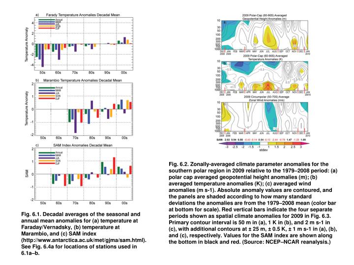
Fig. 6.2. Zonally-averaged climate parameter anomalies for the southern polar region in 2009 relative to the 1979–2008 period: (a) polar cap averaged geopotential height anomalies (m); (b) averaged temperature anomalies (K); (c) averaged wind anomalies (m s-1). Absolute anomaly values are contoured, and the panels are shaded according to how many standard deviations the anomalies are from the 1979–2008 mean (color bar at bottom for scale). Red vertical bars indicate the four separate periods shown as spatial climate anomalies for 2009 in Fig. 6.3. Primary contour interval is 50 m in (a), 1 K in (b), and 2 m s-1 in (c), with additional contours at ± 25 m, ± 0.5 K, ± 1 m s-1 in (a), (b), and (c), respectively. Values for the SAM index are shown along the bottom in black and red. (Source: NCEP–NCAR reanalysis.) Fig. 6.1. Decadal averages of the seasonal and annual mean anomalies for (a) temperature at Faraday/Vernadsky, (b) temperature at Marambio, and (c) SAM index (http://www.antarctica.ac.uk/met/gjma/sam.html). See Fig. 6.4a for locations of stations used in 6.1a–b.
Fig. 6.4. (a) Locations of automatic and manned Antarctic weather stations described in Chapter 6. (b)–(e) 2009 Antarctic climate anomalies at four representative stations (two manned, and two automated). Monthly mean anomalies for temperature (K), MSLP (hPa), and wind speed (m s-1) are shown, with plus signs (+) denoting all-time record anomalies for a given month at each station. Climatological station data starts in 1957 for Amundsen-Scott, 1970 for Marambio (1983 for Marambio wind speeds), and 1980/81 for the AWS records. The base period for calculating the anomalies was 1979–2008 (1980–2008 for the AWS records). Fig. 6.3. (left) Surface pressure anomalies and (right) surface temperature anomaly contours relative to 1979–2008 climatology for (a,b) January–March 2009, (c,d) April–August 2009, and (e,f) September–December 2009. The shaded regions correspond to the number of standard deviations the anomalies are from the 1979–2008 mean, as in Fig. 6.2. (Source: NCEP–NCAR reanalysis.)
Fig. 6.5. Japanese Reanalysis annual precipitation minus evaporation (P-E) and annual mean sea level pressure anomalies: (a) 2009 P-E anomalies, departure from the 1979–2008 mean; (b) 2008 P-E anomalies, departure from the 1979–2007 mean; (c) 2009 annual mean sea level pressure anomalies; and (d) 2008 annual mean sea level pressure anomalies.
Fig. 6.6. Surface snow melt (a) onset date, (b) end date, (c) duration, and (d) melt area for the austral summer 2008/09 melt season.
Fig. 6.8. (a) Ozone hole area versus year from 1979 to 2009. The area is determined by first calculating the area enclosed by the 220 Dobson Unit value over the SH for each day from 21 to 30 September, and then averaging these 10 days. The area of the North American continent is indicated by the horizontal bar (24.71 million km2). (b) Four selected profiles of altitude vs ozone partial pressure (millipascals) measured by ozonesondes at South Pole Station. These 2009 profiles show the pre-ozone hole average in July and August (241 Dobson Units), a mid-September profile and the minimum values of 98 and 101 DU measured at the end of September. (c) Temperature versus year at 50 hPa from 60°S to 75˚S during September. The vertical bars represent the range of values from the individual days of September. The September average over the 1979 to 2009 period is indicated by the horizontal line. Fig. 6.7. (a) Hovmöller diagram of daily satellite-derived sea ice extent anomalies for 2009 (2009 minus the 1979–2008 long-term mean, in 103 km2); (b) and (c) sea ice concentration anomaly maps for April and November 2009, respectively, derived versus the monthly means for 1979–2000 (total anomalies of 1.0 and 0.1 2 x 10⁶ km2, respectively) (courtesy NSIDC; Fetterer et al. 2009); (d) sea ice duration anomaly for 2009, and (e) duration trend (1979–2007). For (d) and (e), see Stammerjohn et al. (2008) for a description of techniques (using daily satellite passive-microwave data). Note that the data used in (d) and (e) are from three different sources: i) 1979–2007 (GSFC Bootstrap dataset, V2); ii) 2008 (F13 Bootstrap daily data); and iii) 2009/10 (NASA Near-Real-Time Sea Ice dataset). However, discrepancies introduced by this factor lead to an uncertainty (difference) level that is well below the magnitude of the large changes/anomalies