Download
1 / 67
670 likes | 998 Views
What is an option?. An option provides the holder with the right to buy or sell a specified quantity of an underlying asset at a fixed price (called a strike price or an exercise price) at or before the expiration date of the option. Since it is a right and not an obligation, the holder can choose

E N D
1. Option Pricing Theory and Applications Aswath Damodaran
2. What is an option? An option provides the holder with the right to buy or sell a specified quantity of an underlying asset at a fixed price (called a strike price or an exercise price) at or before the expiration date of the option.
Since it is a right and not an obligation, the holder can choose not to exercise the right and allow the option to expire.
There are two types of options - call options (right to buy) and put options (right to sell).
3. Call Options A call option gives the buyer of the option the right to buy the underlying asset at a fixed price (strike price or K) at any time prior to the expiration date of the option. The buyer pays a price for this right.
At expiration,
If the value of the underlying asset (S) > Strike Price(K)
Buyer makes the difference: S - K
If the value of the underlying asset (S) < Strike Price (K)
Buyer does not exercise
More generally,
the value of a call increases as the value of the underlying asset increases
the value of a call decreases as the value of the underlying asset decreases
4. Payoff Diagram on a Call
5. Put Options A put option gives the buyer of the option the right to sell the underlying asset at a fixed price at any time prior to the expiration date of the option. The buyer pays a price for this right.
At expiration,
If the value of the underlying asset (S) < Strike Price(K)
Buyer makes the difference: K-S
If the value of the underlying asset (S) > Strike Price (K)
Buyer does not exercise
More generally,
the value of a put decreases as the value of the underlying asset increases
the value of a put increases as the value of the underlying asset decreases
6. Payoff Diagram on Put Option
7. Determinants of option value Variables Relating to Underlying Asset
Value of Underlying Asset; as this value increases, the right to buy at a fixed price (calls) will become more valuable and the right to sell at a fixed price (puts) will become less valuable.
Variance in that value; as the variance increases, both calls and puts will become more valuable because all options have limited downside and depend upon price volatility for upside.
Expected dividends on the asset, which are likely to reduce the price appreciation component of the asset, reducing the value of calls and increasing the value of puts.
Variables Relating to Option
Strike Price of Options; the right to buy (sell) at a fixed price becomes more (less) valuable at a lower price.
Life of the Option; both calls and puts benefit from a longer life.
Level of Interest Rates; as rates increase, the right to buy (sell) at a fixed price in the future becomes more (less) valuable.
8. American versus European options: Variables relating to early exercise An American option can be exercised at any time prior to its expiration, while a European option can be exercised only at expiration.
The possibility of early exercise makes American options more valuable than otherwise similar European options.
However, in most cases, the time premium associated with the remaining life of an option makes early exercise sub-optimal.
While early exercise is generally not optimal, there are two exceptions:
One is where the underlying asset pays large dividends, thus reducing the value of the asset, and of call options on it. In these cases, call options may be exercised just before an ex-dividend date, if the time premium on the options is less than the expected decline in asset value.
The other is when an investor holds both the underlying asset and deep in-the-money puts on that asset, at a time when interest rates are high. The time premium on the put may be less than the potential gain from exercising the put early and earning interest on the exercise price.
9. A Summary of the Determinants of Option Value Factor Call Value Put Value
Increase in Stock Price Increases Decreases
Increase in Strike Price Decreases Increases
Increase in variance of underlying asset Increases Increases
Increase in time to expiration Increases Increases
Increase in interest rates Increases Decreases
Increase in dividends paid Decreases Increases
10. Creating a replicating portfolio The objective in creating a replicating portfolio is to use a combination of riskfree borrowing/lending and the underlying asset to create the same cashflows as the option being valued.
Call = Borrowing + Buying D of the Underlying Stock
Put = Selling Short D on Underlying Asset + Lending
The number of shares bought or sold is called the option delta.
The principles of arbitrage then apply, and the value of the option has to be equal to the value of the replicating portfolio.
11. Option Pricing Model The binomial model is a discrete-time model for asset price movements, with a time interval (t) between price movements.The stock can jump to only one of two points in each time interval, and the option value is estimated iteratively.
As the time interval is shortened, the limiting distribution, as t -> 0, can take one of two forms.
If as t -> 0, price changes become smaller, the limiting distribution is the normal distribution and the price process is a continuous one.
If as t->0, price changes remain large, the limiting distribution is the poisson distribution, i.e., a distribution that allows for price jumps.
The Black-Scholes model applies when the limiting distribution is the normal distribution , and explicitly assumes that the price process is continuous and that there are no jumps in asset prices.
12. The Black-Scholes Model The version of the model presented by Black and Scholes was designed to value European options, which were dividend-protected.
The value of a call option in the Black-Scholes model can be written as a function of the following variables:
S = Current value of the underlying asset
K = Strike price of the option
t = Life to expiration of the option
r = Riskless interest rate corresponding to the life of the option
?2 = Variance in the ln(value) of the underlying asset
13. The Black Scholes Model Value of call = S N (d1) - K e-rt N(d2)
where,
d2 = d1 - ? vt
14. The Normal Distribution
15. Adjusting for Dividends If the dividend yield (y = dividends/ Current value of the asset) of the underlying asset is expected to remain unchanged during the life of the option, the Black-Scholes model can be modified to take dividends into account.
C = S e-yt N(d1) - K e-rt N(d2)
where,
d2 = d1 - ? vt
16. Option Pricing Applications in Equity Valuation Equity in a troubled firm (i.e. a firm with high leverage, negative earnings and a significant chance of bankruptcy) can be viewed as a call option, which is the option to liquidate the firm.
Natural resource companies, where the undeveloped reserves can be viewed as options on the natural resource.
Start-up firms or high growth firms which derive the bulk of their value from the rights to a product or a service (eg. a patent)
17. Limitations of Real Option Pricing Models 1. The underlying asset may not be traded, which makes it difficult to estimate value and variance for the underlying asset.
2. The price of the asset may not follow a continuous process, which makes it difficult to apply option pricing models (like the Black Scholes) that use this assumption.
3. The variance may not be known and may change over the life of the option, which can make the option valuation more complex.
4. Exercise may not be instantaneous, which will affect the value of the option.
18. I. Valuing Equity as an option The equity in a firm is a residual claim, i.e., equity holders lay claim to all cashflows left over after other financial claim-holders (debt, preferred stock etc.) have been satisfied.
If a firm is liquidated, the same principle applies, with equity investors receiving whatever is left over in the firm after all outstanding debts and other financial claims are paid off.
The principle of limited liability, however, protects equity investors in publicly traded firms if the value of the firm is less than the value of the outstanding debt, and they cannot lose more than their investment in the firm.
19. Equity as a call option The payoff to equity investors, on liquidation, can therefore be written as:
Payoff to equity on liquidation = V - D if V > D
= 0 if V = D
where,
V = Value of the firm
D = Face Value of the outstanding debt and other external claims
A call option, with a strike price of K, on an asset with a current value of S, has the following payoffs:
Payoff on exercise = S - K if S > K
= 0 if S = K
20. Payoff Diagram for Liquidation Option
21. Application to valuation: A simple example Assume that you have a firm whose assets are currently valued at $100 million and that the standard deviation in this asset value is 40%.
Further, assume that the face value of debt is $80 million (It is zero coupon debt with 10 years left to maturity).
If the ten-year treasury bond rate is 10%,
how much is the equity worth?
What should the interest rate on debt be?
22. Model Parameters Value of the underlying asset = S = Value of the firm = $ 100 million
Exercise price = K = Face Value of outstanding debt = $ 80 million
Life of the option = t = Life of zero-coupon debt = 10 years
Variance in the value of the underlying asset = ?2 = Variance in firm value = 0.16
Riskless rate = r = Treasury bond rate corresponding to option life = 10%
23. Valuing Equity as a Call Option Based upon these inputs, the Black-Scholes model provides the following value for the call:
d1 = 1.5994 N(d1) = 0.9451
d2 = 0.3345 N(d2) = 0.6310
Value of the call = 100 (0.9451) - 80 exp(-0.10)(10) (0.6310) = $75.94 million
Value of the outstanding debt = $100 - $75.94 = $24.06 million
Interest rate on debt = ($ 80 / $24.06)1/10 -1 = 12.77%
24. The Effect of Catastrophic Drops in Value Assume now that a catastrophe wipes out half the value of this firm (the value drops to $ 50 million), while the face value of the debt remains at $ 80 million. What will happen to the equity value of this firm?
It will drop in value to $ 25.94 million [ $ 50 million - market value of debt from previous page]
It will be worth nothing since debt outstanding > Firm Value
It will be worth more than $ 25.94 million
25. Valuing equity in a troubled firm The first implication is that equity will have value, even if the value of the firm falls well below the face value of the outstanding debt.
Such a firm will be viewed as troubled by investors, accountants and analysts, but that does not mean that its equity is worthless.
Just as deep out-of-the-money traded options command value because of the possibility that the value of the underlying asset may increase above the strike price in the remaining lifetime of the option, equity will command value because of the time premium on the option (the time until the bonds mature and come due) and the possibility that the value of the assets may increase above the face value of the bonds before they come due.
26. Illustration : Value of a troubled firm Assume now that, in the previous example, the value of the firm were reduced to $ 50 million while keeping the face value of the debt at $80 million.
This firm could be viewed as troubled, since it owes (at least in face value terms) more than it owns.
The equity in the firm will still have value, however.
27. Valuing Equity in the Troubled Firm Value of the underlying asset = S = Value of the firm = $ 50 million
Exercise price = K = Face Value of outstanding debt = $ 80 million
Life of the option = t = Life of zero-coupon debt = 10 years
Variance in the value of the underlying asset = ?2 = Variance in firm value = 0.16
Riskless rate = r = Treasury bond rate corresponding to option life = 10%
28. The Value of Equity as an Option Based upon these inputs, the Black-Scholes model provides the following value for the call:
d1 = 1.0515 N(d1) = 0.8534
d2 = -0.2135 N(d2) = 0.4155
Value of the call = 50 (0.8534) - 80 exp(-0.10)(10) (0.4155) = $30.44 million
Value of the bond= $50 - $30.44 = $19.56 million
The equity in this firm drops by, because of the option characteristics of equity.
This might explain why stock in firms, which are in Chapter 11 and essentially bankrupt, still has value.
29. Equity value persists ..
30. Would you take this project? Assume now that you are the manager of the firm, hired by and compensated by the equity investors. If your objective were firm value maximization, would you take on a project with a negative net present value of $ 2 million?
Yes
No
Would you change your mind if I told you that this was a very risky project with a negative net present value of $ 2 million?
Yes
No
31. The Conflict between bondholders and stockholders Stockholders and bondholders have different objective functions, and this can lead to conflicts between the two.
For instance, stockholders have an incentive to take riskier projects than bondholders do, and to pay more out in dividends than bondholders would like them to.
This conflict between bondholders and stockholders can be illustrated dramatically using the option pricing model.
Since equity is a call option on the value of the firm, an increase in the variance in the firm value, other things remaining equal, will lead to an increase in the value of equity.
It is therefore conceivable that stockholders can take risky projects with negative net present values, which while making them better off, may make the bondholders and the firm less valuable. This is illustrated in the following example.
32. Illustration: Effect on value of the conflict between stockholders and bondholders Consider again the firm described in the earlier example , with a value of assets of $100 million, a face value of zero-coupon ten-year debt of $80 million, a standard deviation in the value of the firm of 40%. The equity and debt in this firm were valued as follows:
Value of Equity = $75.94 million
Value of Debt = $24.06 million
Value of Firm == $100 million
Now assume that the stockholders have the opportunity to take a project with a negative net present value of -$2 million, but assume that this project is a very risky project that will push up the standard deviation in firm value to 50%.
33. Valuing Equity after the Project Value of the underlying asset = S = Value of the firm = $ 100 million - $2 million = $ 98 million (The value of the firm is lowered because of the negative net present value project)
Exercise price = K = Face Value of outstanding debt = $ 80 million
Life of the option = t = Life of zero-coupon debt = 10 years
Variance in the value of the underlying asset = s2 = Variance in firm value = 0.25
Riskless rate = r = Treasury bond rate corresponding to option life = 10%
34. Option Valuation Option Pricing Results for Equity and Debt Value
Value of Equity = $77.71
Value of Debt = $20.29
Value of Firm = $98.00
The value of equity rises from $75.94 million to $ 77.71 million , even though the firm value declines by $2 million. The increase in equity value comes at the expense of bondholders, who find their wealth decline from $24.06 million to $20.19 million.
35. Effects of an Acquisition Assume that you are the manager of a firm and that you buy another firm, with a fair market value of $ 150 million, for exactly $ 150 million. In an efficient market, the stock price of your firm will
Increase
Decrease
Remain Unchanged
36. II. Effects on equity of a conglomerate merger You are provided information on two firms, which operate in unrelated businesses and hope to merge.
Firm A Firm B
Value of the firm $100 million $ 150 million
Face Value of Debt $ 80 million $ 50 million (Zero-coupon debt)
Maturity of debt 10 years 10 years
Std. Dev. in value 40 % 50 %
Correlation between cashflows 0.4
The ten-year bond rate is 10%.
The variance in the value of the firm after the acquisition can be calculated as follows:
Variance in combined firm value = w12 s12 + w22 s22 + 2 w1 w2 r12s1s2
= (0.4)2 (0.16) + (0.6)2 (0.25) + 2 (0.4) (0.6) (0.4) (0.4) (0.5)
= 0.154
37. Valuing the Combined Firm The values of equity and debt in the individual firms and the combined firm can then be estimated using the option pricing model:
Firm A Firm B Combined firm
Value of equity in the firm $75.94 $134.47 $ 207.43
Value of debt in the firm $24.06 $ 15.53 $ 42.57
Value of the firm $100.00 $150.00 $ 250.00
The combined value of the equity prior to the merger is $ 210.41 million and it declines to $207.43 million after.
The wealth of the bondholders increases by an equal amount.
There is a transfer of wealth from stockholders to bondholders, as a consequence of the merger. Thus, conglomerate mergers that are not followed by increases in leverage are likely to see this redistribution of wealth occur across claim holders in the firm.
38. Obtaining option pricing inputs - Some real world problems The examples that have been used to illustrate the use of option pricing theory to value equity have made some simplifying assumptions. Among them are the following:
(1) There were only two claim holders in the firm - debt and equity.
(2) There is only one issue of debt outstanding and it can be retired at face value.
(3) The debt has a zero coupon and no special features (convertibility, put clauses etc.)
(4) The value of the firm and the variance in that value can be estimated.
39. Real World Approaches to Getting inputs
40. Valuing Equity as an option - The example of an airline The airline owns routes in North America and Europe , as well as other assets, with the following estimates of current market value:
North America $ 400 million
Europe $ 500 million
Other Assets $ 300 million
The airline has considerable debt outstanding. It has four debt issues outstanding with the following characteristics:
Maturity Face Value Coupon Duration
20 year debt $ 100 mil 11% 14.1 years
15 year debt $ 100 mil 12% 10.2 years
10 year debt $ 200 mil 12% 7.5 years
1 year debt $ 800 mil 12.5% 1 year
41. More inputs The stock of the airline has been trading on the NYSE. The annualized standard deviation in ln(stock prices) has been 25%, and the firm's debt has been approximately 90% of the firm value (during the variance estimation period).
The firm is rated B. Though its bonds are not traded, other B rated bonds have had an annualized standard deviation of 10% (in ln(bond prices)). The correlation between B rated bonds and this airline's stock price is 0.3.
The firm pays no dividends. The current T. Bond rate is 8%.
42. Valuing Equity in the Airline Step 1: Estimate the value of the firm = Sum of the value of its assets = 400 + 500 + 300 = 1,200 million
Step 2: Estimate the average duration of the debt outstanding = (100/1200) * 14.1 + (100/1200) * 10.2 + (200/1200) * 7.5 + (800/1200) * 1 = 3.9417 years
Step 3: Estimate the face value of debt outstanding = 100 + 100 + 200 + 800 = 1,200 million: Add cumulated coupons on the debt to this amount: (11*20+12*15+24*10+100*1) = 740 million
Step 4: Estimate the variance in the value of the firm
Variance= (E/(D+E))2 ?e2 + (D/(D+E))2 ?d2 + 2 (E/(D+E)) (D/(D+E)) ?ed??e??d
= (.1)2 (.25)2 + (.9)2 (.10)2 + 2 (.1)(.9)(.3) (.25)(.10) = 0.010075
Step 5: Value equity as an option
d1 = -0.7285 N(d1) = 0.2332
d2 = -0.9278 N(d2) = 0.1769
Equity = 1200 (0.2332) - 1940 exp(-0.08)(3.9417) (0.1769) = $ 29.53 mil
43. Valuing Equity as an option - Cablevision Systems Cablevision Systems was a firm in trouble in March 1995.
The book value of equity in March 1995 was negative : - 1820 million
It lost $315 million in 1994 and was expected to lose equivalent amounts in 1995 and 1996.
It had $ 3000 million in face value debt outstanding (with coupons)
The weighted average duration of this debt was 4.62 years
Debt Type Face Value Duration
Short term Debt $ 865 mil 0.5 years
Bank Debt $ 480 mil 3.0 years
Senior Debt $ 832 mil 6.0 years
Senior Subordinated $ 823 mil 8.5 years
Total $ 3000 mil 4.62 years
The face values of the debt include the cumulated coupon payments on each.
44. The Basic DCF Valuation The value of the firm estimated using projected cashflows to the firm, discounted at the weighted average cost of capital was $2,887 million.
This was based upon the following assumptions �
Revenues will grow 14% a year for the next 5 years, and make a linear transition to 5% in 10 years.
The COGS which is currently 69% of revenues will drop to 65% of revenues in yr 5 and stay at that level. (68% in 1996, 67% in 1997, 66% in 1998, 65% in 1999)
Capital spending and depreciation will grow 10% a year for the next five yearsafter which the growth rate will drop to 5% a year.
Working capital will remain at 5% of revenues.
The debt ratio, which is currently 70.14%, will drop to 50% after year 10. The cost of debt is 10% in high growth period and 8.5% after that.
The beta for the stock will be 1.55 for the next five years, and drop to 1.1 over the next 5 years.
The treasury bond rate is 7.5%.
45. Other Inputs The stock has been traded on the NYSE, and the variance based upon ln (monthly prices) between 1990 and 1994 is 0.0133.
There are Cablevision bonds(due 2002), that were traded from 1990 to 1994, and the variance in ln(monthly price)s for these bonds is 0.0012.
The correlation between stock and bond price changes is 0.25. The proportion of debt during the period (1990-94) was 70%.
The stock and bond price variance are first annualized:
Annualized variance in stock price = 0.0133 * 12 = 0.16 s= 0.40
Annualized variance in bond price = 0.0012 * 12 = 0.0144 s= 0.12
Annualized variance in firm value
= (0.30)2 (0.16) + (0.70)2 (0.0.0144) + 2 (0.3) (0.7)(0.25)(0.40)(0.12)= 0.02637668
The five-year bond rate (corresponding to the weighted average duration of 4.62 years) is 7%.
46. Valuing Cablevision Equity Inputs to Model
Value of the underlying asset = S = Value of the firm = $ 2887 million
Exercise price = K = Face Value of outstanding debt = $ 3000 million
Life of the option = t = Weighted average duration of debt = 4.62 years
Variance in the value of the underlying asset = ?2 = Variance in firm value = 0.0264
Riskless rate = r = Treasury bond rate corresponding to option life = 7%
Based upon these inputs, the Black-Scholes model provides the following value for the call:
d1 = 0.9910 N(d1) = 0.8391
d2 = 0.6419 N(d2) = 0.7391
Value of the call = 2887 (0.8391) - 3000 exp(-0.07)(4.62) (0.7395) = $ 817 million
47. II. Valuing Natural Resource Options/ Firms In a natural resource investment, the underlying asset is the resource and the value of the asset is based upon two variables - the quantity of the resource that is available in the investment and the price of the resource.
In most such investments, there is a cost associated with developing the resource, and the difference between the value of the asset extracted and the cost of the development is the profit to the owner of the resource.
Defining the cost of development as X, and the estimated value of the resource as V, the potential payoffs on a natural resource option can be written as follows:
Payoff on natural resource investment = V - X if V > X
= 0 if V= X
48. Payoff Diagram on Natural Resource Firms
49. Estimating Inputs for Natural Resource Options
50. Valuing an Oil Reserve Consider an offshore oil property with an estimated oil reserve of 50 million barrels of oil, where the present value of the development cost is $12 per barrel and the development lag is two years.
The firm has the rights to exploit this reserve for the next twenty years and the marginal value per barrel of oil is $12 per barrel currently (Price per barrel - marginal cost per barrel).
Once developed, the net production revenue each year will be 5% of the value of the reserves.
The riskless rate is 8% and the variance in ln(oil prices) is 0.03.
51. Inputs to Option Pricing Model Current Value of the asset = S = Value of the developed reserve discounted back the length of the development lag at the dividend yield = $12 * 50 /(1.05)2 = $ 544.22
(If development is started today, the oil will not be available for sale until two years from now. The estimated opportunity cost of this delay is the lost production revenue over the delay period. Hence, the discounting of the reserve back at the dividend yield)
Exercise Price = Present Value of development cost = $12 * 50 = $600 million
Time to expiration on the option = 20 years
Variance in the value of the underlying asset = 0.03
Riskless rate =8%
Dividend Yield = Net production revenue / Value of reserve = 5%
52. Valuing the Option Based upon these inputs, the Black-Scholes model provides the following value for the call:
d1 = 1.0359 N(d1) = 0.8498
d2 = 0.2613 N(d2) = 0.6030
Call Value= 544 .22 exp(-0.05)(20) (0.8498) -600 (exp(-0.08)(20) (0.6030)= $ 97.08 million
This oil reserve, though not viable at current prices, still is a valuable property because of its potential to create value if oil prices go up.
53. Extending the option pricing approach to value natural resource firms Since the assets owned by a natural resource firm can be viewed primarily as options, the firm itself can be valued using option pricing models.
The preferred approach would be to consider each option separately, value it and cumulate the values of the options to get the firm value.
Since this information is likely to be difficult to obtain for large natural resource firms, such as oil companies, which own hundreds of such assets, a variant is to value the entire firm as one option.
A purist would probably disagree, arguing that valuing an option on a portfolio of assets (as in this approach) will provide a lower value than valuing a portfolio of options (which is what the natural resource firm really own). Nevertheless, the value obtained from the model still provides an interesting perspective on the determinants of the value of natural resource firms.
54. Inputs to the Model Input to model Corresponding input for valuing firm
Value of underlying asset Value of cumulated estimated reserves of the resource owned by the firm, discounted back at the dividend yield for the development lag.
Exercise Price Estimated cumulated cost of developing estimated reserves
Time to expiration on option Average relinquishment period across all reserves owned by firm (if known) or estimate of when reserves will be exhausted, given current production rates.
Riskless rate Riskless rate corresponding to life of the option
Variance in value of asset Variance in the price of the natural resource
Dividend yield Estimated annual net production revenue as percentage of value of the reserve.
55. Valuing Gulf Oil Gulf Oil was the target of a takeover in early 1984 at $70 per share (It had 165.30 million shares outstanding, and total debt of $9.9 billion).
It had estimated reserves of 3038 million barrels of oil and the average cost of developing these reserves was estimated to be $10 a barrel in present value dollars (The development lag is approximately two years).
The average relinquishment life of the reserves is 12 years.
The price of oil was $22.38 per barrel, and the production cost, taxes and royalties were estimated at $7 per barrel.
The bond rate at the time of the analysis was 9.00%.
Gulf was expected to have net production revenues each year of approximately 5% of the value of the developed reserves. The variance in oil prices is 0.03.
56. Valuing Undeveloped Reserves Value of underlying asset = Value of estimated reserves discounted back for period of development lag= 3038 * ($ 22.38 - $7) / 1.052 = $42,380.44
Exercise price = Estimated development cost of reserves = 3038 * $10 = $30,380 million
Time to expiration = Average length of relinquishment option = 12 years
Variance in value of asset = Variance in oil prices = 0.03
Riskless interest rate = 9%
Dividend yield = Net production revenue/ Value of developed reserves = 5%
Based upon these inputs, the Black-Scholes model provides the following value for the call:
d1 = 1.6548 N(d1) = 0.9510
d2 = 1.0548 N(d2) = 0.8542
Call Value= 42,380.44 exp(-0.05)(12) (0.9510) -30,380 (exp(-0.09)(12) (0.8542)= $ 13,306 million
57. Valuing Gulf Oil In addition, Gulf Oil had free cashflows to the firm from its oil and gas production of $915 million from already developed reserves and these cashflows are likely to continue for ten years (the remaining lifetime of developed reserves).
The present value of these developed reserves, discounted at the weighted average cost of capital of 12.5%, yields:
Value of already developed reserves = 915 (1 - 1.125-10)/.125 = $5065.83
Adding the value of the developed and undeveloped reserves
Value of undeveloped reserves = $ 13,306 million
Value of production in place = $ 5,066 million
Total value of firm = $ 18,372 million
Less Outstanding Debt = $ 9,900 million
Value of Equity = $ 8,472 million
Value per share = $ 8,472/165.3 = $51.25
58. Valuing product patents as options A product patent provides the firm with the right to develop the product and market it.
It will do so only if the present value of the expected cash flows from the product sales exceed the cost of development.
If this does not occur, the firm can shelve the patent and not incur any further costs.
If I is the present value of the costs of developing the product, and V is the present value of the expected cashflows from development, the payoffs from owning a product patent can be written as:
Payoff from owning a product patent = V - I if V> I
= 0 if V = I
59. Payoff on Product Option
60. Obtaining Inputs for Patent Valuation
61. Valuing a Product Patent Assume that a firm has the patent rights, for the next twenty years, to a product which
requires an initial investment of $ 1.5 billion to develop,
and a present value, right now, of cash inflows of only $1 billion.
Assume that a simulation of the project under a variety of technological and competitive scenarios yields a variance in the present value of inflows of 0.03.
The current riskless twenty-year bond rate is 10%.
62. Valuing the Option Value of the underlying asset = Present value of inflows (current) = $1,000 million
Exercise price = Present value of cost of developing product = $1,500 million
Time to expiration = Life of the patent = 20 years
Variance in value of underlying asset = Variance in PV of inflows = 0.03
Riskless rate = 10%
Based upon these inputs, the Black-Scholes model provides the following value for the call:
d1 = 1.1548 N(d1) = 0.8759
d2 = 0.3802 N(d2) = 0.6481
Call Value= 1000 exp(-0.05)(20) (0.8759) -1500 (exp(-0.10)(20) (0.6481)= $ 190.66 million
63. Implications This suggests that though this product has a negative net present value currently, it is a valuable product when viewed as an option. This value can then be added to the value of the other assets that the firm possesses, and provides a useful framework for incorporating the value of product options and patents.
Product patents will increase in value as the volatility of the sector increases.
Research and development costs can be viewed as the cost of acquiring these options.
64. Valuing Biogen The firm is receiving royalties from Biogen discoveries (Hepatitis B and Intron) at pharmaceutical companies. These account for FCFE per share of $1.00 and are expected to grow 10% a year until the patent expires (in 15 years).
Using a beta of 1.1 to value these cash flows (leading to a cost of equity of 13.05%), we arrive at a present value per share:
Value of Existing Products = $ 12.14
65. Valuing the Other Component: Avonex The firm also has a patent on Avonex, a drug to treat multiple sclerosis, for the next 17 years, and it plans to produce and sell the drug by itself. The key inputs on the drug are as follows:
Present Value of Cash Flows from Introducing the Drug Now = S = $ 3.422 billion
Present Value of Cost of Developing Drug for Commercial Use = K = $ 2.875 billion
Patent Life = t = 17 years Riskless Rate = r = 6.7% (17-year T.Bond rate)
Variance in Expected Present Values =s2 = 0.224 (Industry average firm variance for bio-tech firms)
Expected Cost of Delay = y = 1/17 = 5.89%
d1 = 1.1362 N(d1) = 0.8720
d2 = -0.8512 N(d2) = 0.2076
Call Value= 3,422 exp(-0.0589)(17) (0.8720) - 2,875 (exp(-0.067)(17) (0.2076)= $ 907 million
Call Value per Share from Avonex = $ 907 million/35.5 million = $ 25.55
66. Biogen�s total value per share Value of Existing Products = $ 12.14
Call Value per Share from Avonex = $ 907 million/35.5 million = $ 25.55
Biogen Value Per Share = Value of Existing Assets + Value of Patent = $ 12.14 + $ 25.55 = $ 37.69