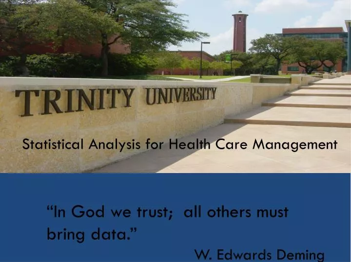
Data-Driven Decision Making Ed Schumacher, Ph.D.

Data-Driven Decision MakingEd Schumacher, Ph.D. Statistical Analysis for Health Care Management CENTENE-TRINITY-OLIN “In God we trust; all others must bring data.” W. Edwards Deming

Creative Destruction of Medicine New Medicine (individual-based) Consumerism Social Networking Wireless Censors Super Convergence Genomics New financing models Imaging Predictive Analytics Information Systems Computing Power + Big Data Old Medicine (population-based)

Thinking Like a Statistician • The World is made up of information • We make judgments and decisions based on the data that reaches us • If that data is systematically biased then these judgments are systematically wrong • Formal statistical analysis provides precise ways to convert data into information • But we can also use these concepts to help us in our day-to-day thinking

Start with a Story • A study of the incidence of kidney cancer in the 3,141 counties of the US reveals a remarkable pattern. The counties with the lowest incidence of kidney cancer are: • Rural, sparsely populated, located in traditionally Republican states in the midwest, south, and west.

We are not natural statisticians • We like stories • A good story usually trumps good data • This causes us to make mistakes in evaluating the randomness of truly random events • Which of these is more likely? • BBBGGG • GGGGGG • BGBGBG

We misunderstand randomness • We pay more attention to the content of messages than to information about their reliability • We end up with a view of the world that is simpler and more coherent than the data justify • Many facts of the world are due to chance • Causal explanation of chance events are inevitably wrong • Even faced with data to the contrary, we stick to our story • Emulate successful firms

So we need to train our brains to think statistically • Huge quantities of data, from an increasingly variety of sources • Key is to convert data into information. • A basic understanding of statistical concepts is critical

Selection Bias • We make a lot of decisions based on incomplete information • Often we make inference about a whole population based on a subset of that population • As long as the subset is representative of the whole, your inferences will be reasonable • But if our subset is a special set of the population, then we can be way off

Selection Bias • Suppose you are in charge of monitoring sound quality in a large auditorium that is filled with people Can Hear a Little Can Hear Everything Can’t Hear Anything

Selection Bias • After the lecture you told people to go to a certain web site and fill out a survey on how well they could hear Can Hear Everything Can Hear a Little Can’t Hear Anything

Selection Bias • Or what you get back looks as follows. What do we conclude about the sound? Can Hear a Little Can Hear Everything

Selection Bias • Where do we see selection bias?

Selection Bias • The Feedback Effect • My favorite professor • Teaching evaluations • Leaders often have skewed impressions of their organizations • If there are real or perceived dangers to expressing a negative opinion • Many instances of “supervisory madness” are not the result of malice or idiocy, but rather selection bias • Fox News vs MSNBC, NYTimes vs WSJ • Geographic variations in health care • Spending at the end of life • Other instances were we receive “first person” information

The Filter Bubble = Selection Bias

Endogeneity – Correlation Does not Imply Causation • Endogeneity • Not even a word according to Microsoft • Basic idea: • We assume X Y but in fact Y X • Or Assume A B but in fact C A and C B

Endogeneity • Omitted Variable Bias • It is typically assumed that GPA is a good measure of a job or graduate school applicant’s prospects • GPA is a function of how hard you work and how able you are • X converts effort into GPA points • Y converts ability into GPA points • Error is a term that allows for random variations

Endogeneity • Problem: • Students can pick their courses • Now the error term is not random – it is correlated with an omitted variable: the difficulty of the course • Taking easier courses results in a higher GPA • So our X and Y effects get diluted • We may not write out equations like this very often, but we implicitly do in our heads. • Need to be aware of omitted variables

Endogeneity • Causality Loops -- or reverse causation • Does X cause Y or does Y cause X? Or BOTH? • Open That Bottle Night

Endogeneity • Her equation Computer time is a function of football time • My equation Football time is a function of computer time • Both variables are endogeneous to the other • The surgeries don’t start on time because the anesthesiologist doesn’t show up on time • The anesthesiologist doesn’t show up on time because the surgeries don’t start on time

Endogeneity • A similar problem shows up in much advertising: • People who switched to Progressive save $$$$ • Note the big endogeneity problem here • The decision to switch insurance is endogeneous – people who discover they would save money will switch, those who discover they won’t tend not to switch. • The company wants you to think switching will save: X*Switch = Savings + error – switching causes savings But: Y*Savings = Switch + error – savings causes switching

Endogeneity • “Mark Zuckerberg dropped out of college and did well for himself– we need to encourage our youth to be more adventurous, risk-taking, entrepreneurial” Taking risk results in a higher chance of success. But… Being successful makes it more likely to drop out • Note also there is a sample selection problem here

Endogeneity • Challenge of the Big Data movement • The idea is to move away from causation and towards correlation • “Correlations are powerful not only because they offer insights, but also because the insights they offer are relatively clear. These insights often get obscured when we bring causality back into the picture” -- Mayer-Schonberger and Cukier, Big Data

Endogeneity • Big Data has made some impressive observations: • Google search terms and flu outbreaks • Farecast – predicting if the price of plane tickets will rise or fall in the future • Target knows you are pregnant before your family does • Wal-Mart: hurricanes and strawberry Pop-Tarts • But there are some limits

Endogeneity • Correlations are not always all that clear • A zillion things can correlate with the other. • Ice cream sales and drowning are highly correlated • You will have to rely on some causal hypothesis • We are “blind to randomness” – Black Swans • The passing of time can produce gigantic and unpredictable changes in taste and behavior • These changes will be poorly anticipated by looking at patterns of data on what just happened

Endogeneity • Data creates bigger haystacks • As we acquire more data we have the ability to find many more statistically significant correlations • Most of these correlations are spurious • Falsity grows exponentially the more data we collect • The haystack gets bigger but the needle stays the same

Endogeneity • Big Data is a tool – a good tool but just a tool • It is really good at telling you what to pay attention to, but then you need to get back to the world of causality to benefit. • “Big data is like the offensive coordinator up in the booth at a football game who, with altitude, can see patterns others miss. But the head coach and players still need to be on the field of subjectivity” David Brooks

Bayes' Theorem • Student in middle school • “given I received this note, what are the chances she actually likes me?” • This is what is known as conditional probability • The note is the conditioning event • The probability I am interested in is “does she like me?” • How do we update when we receive new information?

Bayes' Theorem • Bayes' Theorem gives us the answer. We need 3 quantities • The probability of getting a note conditional on her liking me -- let’s say this is 75% • The probability of getting a note conditional on her NOT liking me – let’s say this is 20% • Prior probability – what is the chance of her liking me prior to the note appearing? Let’s say 10%

Bayes' Theorem • So now we can calculate the probability of her liking me conditional on receiving the note:

Bayes' Theorem • Note the power of the prior belief. Suppose we put a 50% chance on her liking me prior to the note • That raises the probability of her liking me conditional on getting the note to almost 80% • I’ll come back to this in a bit, but our priors matter

Bayes' Theorem • Application – Screening for breast cancer among women in their 40s. • What is the probability of getting cancer conditional on getting a positive mammogram?

Bayes' Theorem • The prior probability of a woman in her 40s developing breast cancer is about 1.4% • If a woman does not have cancer, a mammogram will incorrectly claim she does about 10% of the time • If a woman does have cancer a mammogram will detect it about 75% of the time

Bayes' Theorem • So the probability of having breast cancer conditional on a positive mammogram is:

Bayes' Theorem • Even though false positives are not too likely, they dominate since the prior probability is so low. • To see this assume a population of 1000 women in their 40s • 14 of them will have cancer, 986 will not • If there is a 10% chance of a false positive -- 98.6 will have false positives • If there is a 75% chance of a true positive --10.5 will have true positives • Thus 109.1 women will have positive mammograms, 10.5 of them will have cancer: 10.5/109.1=.096

Bayes' Theorem • This is known as the Base-Rate Fallacy • We tend to be very bad at using Bayes' Theorem and tend to focus on the most immediate information • The value of Bayes' theorem is that it allows us to account for our prior beliefs but then to update them with this new information • Bayes' helps us understand why two people can look at the same data and come to two opposite conclusions:

Bayes' Theorem

Bayes' Theorem • But the encouraging thing about Bayes' Theorem is that over time our beliefs should converge as we update with new information

Descriptive Statistics • Descriptive Statistics vs. Inferential Statistics – Descriptive stats are used to summarize and describe a group of data. • The analyst is neutral • Inferential statistics makes possible the estimation of a characteristic of a population based only on sample results • Analyst uses judgment

Measures of Central Tendency • Consider the following data

Mean, Median, Mode • Three common measures of central tendency: Mean Median and Mode • Arithmetic Mean: • Where is the sample mean • n is the number of observations in the sample • xi is the ith observation of the variable x • Xi is the summation of all Xi values in the sample • (5+5+2+10+4+5+3)/7 = 4.86 • The average LOS is 4.86 days for this sample

Geometric Mean • An alternative to the arithmetic mean – often used when there are positive outliers. • Or • The log of the geometric mean is equal to the log mean • The geometric mean is always less than the arithmetic mean

Median • The median is the middle value in an ordered array of data. • If there are no ties, half the observations will be smaller than the median and half will be larger. • The median is unaffected by any extreme observations in a set of data So 5 is the median

Mode • The mode is the value in a set of data that appears most frequently. • So the mode is 5 in our sample

Measures of Variation • Range • The range is the difference between the largest and smallest observations in the data. In our hospital revenue data the range is 10-2=8. • The Interquartile Range • The interquartile range is obtained by subtracting the first quartile from the third quartile.

Variance • The sample variance is roughly the average of the squared differences between each of the observations in a set of data and the mean: • So for our data we would get: 6.48 days • Why n-1?

Standard Deviation • If we take the square root of the variance we get the standard deviation: • S = S2 • So S = 2.54 • On average each patient’s stay is about 2.5 days away from the average LOS. • Note that in the squaring process, observations that are further from the mean get more weight than are observations that are closer to the mean.

Coefficient of Variation • The coefficient of variation is a relative measure of variation: • This statistic is most useful when making comparisons across different types of data that might use different scales or different units of measurement. • It makes it easier to compare apples to oranges.

Coefficient of Variation • Wait times for 3 different lab tests:

Correlation Coefficient • The correlation coefficient gives a value to how to continuous variables relate to each other.

Data-Driven Decision Making Ed Schumacher, Ph.D.