Download
1 / 16
160 likes | 193 Views
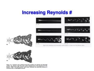
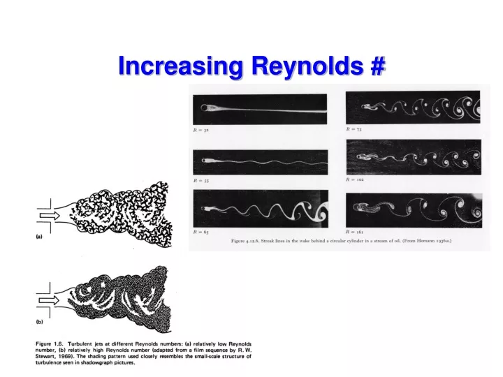
Increasing Reynolds #. Turbulence characteristics. 3-dimensional rotational – carries vorticity (unlike linear surface waves) irregular, unpredictable (random) motion – described by probability density function diffusive – several orders of magnitude greater than molecular diffusion

E N D
Turbulence characteristics 3-dimensional rotational – carries vorticity (unlike linear surface waves) irregular, unpredictable (random) motion – described by probability density function diffusive – several orders of magnitude greater than molecular diffusion dissipative – K.E.→ heatrequires steady supply of energy
Turbulence characteristics flow has large Reynolds #,(nonlinear) does not obey a dispersion relation (not wavelike) broad wavenumber spectrum generally anisotropic at larger scales is a function of the flow, not the fluid satisfies Navier-Stokes equations
Dynamic Stability Concepts Figure from Thorpe Statically stable, dynamically unstable = forced convection (figure from Stull)
Vertical turbulent transports What is a turbulent flux? Reynolds’ decomposition: <wT> = <w><T> + <w’T’> What determines the vertical distribution of turbulence? TKE equation: dTKE/dt = production – dissipation + advection How does turbulence determine the interfacial fluxes of heat, moisture and momentum? Near-surface gradients and TKE levels are related. How are vertical turbulent transports modeled? Flux profile relationships (Monin-Obukhov similarity theory) closure schemes (parameterizations) layered versus level models
Turbulent Flux Definitions Reference Lecture 2 for bulk parameterizations of these
PBL TKE budget forced convection free convection • u* friction velocity • w* convective velocity scale • h boundary layer height • ε dissipation of TKE • S shear production of TKE • B buoyancy production/damping of TKE • T transport of TKE
the flow is in steady state, i.e, • the boundary layer is horizontally homogeneous, i.e., and • the boundary layer is statically neutral, i.e., • the boundary layer is barotropic, i.e., Ug and Vg are constant with height • there is no subsidence, i.e., W = 0 Ekman Flow assumptions
(1) • How can we solve equation set (1)? • First, let's define the magnitude of the geostrophic wind, G by G = [U2g + V2g]0.5 • Let's also assume that the geostrophic wind is parallel to the X axis, thus: • G = Ug • V2g = 0 • Let's also use first-order local closure K-theory, assuming a constant Kmto eliminate the flux terms. • Hence: (2) • Substituting (2) into (1) gives: • (3) Ekman Flow
Here we have a set of two partial differential equations...., how to solve????? • Well, we need to specify the boundary conditions: • U= 0 at z = 0 • V= 0 at z = 0 • U --> G as z --> large (get above the boundary layer) • V --> 0 as z --> large (the geostrophic flow above the boundary layer is parallel to the X axis) • The solution to (3) using the above boundary conditions is: • (4) • where Ekman Flow