Download

1 / 94
950 likes | 1.05k Views
第 3 章 Fuzzy Identification and Estimation. 教学内容:. 这一章主要研究了怎样用模糊进行评估和辨识。模糊辨识设计的最主要的问题是怎样用已知的离散数据构建一个模糊系统。首先介绍最基本的函数近似问题,然后介绍了传统的辨识方法:最小二乘法即怎样用批量最小二乘法和递归最小二乘法来辨识一个系统以匹配输入输出数据。最后讲述用这两种方法直接训练模糊系统。

E N D
教学内容: • 这一章主要研究了怎样用模糊进行评估和辨识。模糊辨识设计的最主要的问题是怎样用已知的离散数据构建一个模糊系统。首先介绍最基本的函数近似问题,然后介绍了传统的辨识方法:最小二乘法即怎样用批量最小二乘法和递归最小二乘法来辨识一个系统以匹配输入输出数据。最后讲述用这两种方法直接训练模糊系统。 • 本章将现代控制理论的自适应控制理论应用于模糊控制技术中,以期提高模糊控制系统的动态、静态性能,增强模糊控制系统对于模型的参数、结构变化的鲁棒性以及控制系统不同相应阶段对控制其性能的不同要求,提高控制系统的综合品质。
主要内容: • 直接自适应控制和间接自适应控制的基本概念; • 模糊模型参考学习控制( FMRLC )的原理、结构; • FMRLC 的设计和实现。
教学重点: • 详细阐述了用一个函数拟和输入输出数据所应注意的问题,同时还阐述了怎样将语言变量信息转化为函数,以便用该函数来拟和输入输出数据。其中输入输出数据的选择关系着辨识结果的好坏,通常要求其能对系统充分激励。 • 模糊模型参考学习控制(FMRLC)的原理和结构 。
教学难点: • 对FMRLC中学习机制的准确把握和理解,关键是模糊逆模型的设计。
教学要求: • 本章的学习需要预先掌握一定的自适应控制、自校正调节器的基础知识、概念。要求掌握模糊模型参考学习控制(FMRLC)的原理和结构。 • 当离散数据是通过试验获得的输入输出数据的时候,我们就可以通过数据来辨识一个模糊系统的模型;当数据是通过其它的途径获得时,可以对数据进行插补处理,然后用处理过的数据来辨识模糊系统。
3.1 Overview • While up to this point we have focused on control, in this chapter we will examine how to use fuzzy systems for estimation and identification. The basic problem to be studied here is how to construct a fuzzy system from numerical data. This is in contrast to our discussion in Chapters 2 and 3, where we used linguistics as the starting point to specify a fuzzy system. If the numerical data is plant input-output data obtained from an experiment, we may identify a fuzzy system model of the plant. This may be useful for simulation purposes and sometimes for use in a controller. On the other hand, the data may come from other sources, and a fuzzy system may be used to provide for a parameterized nonlinear function that fits the data by using its basic interpolation capabilities. For instance, suppose that we have a human expert who controls some process and we observe how she or he does this by observing what numerical plant input the expert picks for the given numerical data that she or he observes. Suppose further that we have many such associations between "decision-making data." The methods in this chapter will show how to construct rules for a fuzzy controller from this data (i.e., identify a controller from the human-generated decision-making data), and in this sense they provide another method to design controllers.
Yet another problem that can be solved with the methods in this chapter is that of how to construct a fuzzy system that will serve as a parameter estimator. To do this, we need data that shows, roughly how the input-output mapping of the estimator should behave (i.e., how it should estimate). One way to generate this data is to begin by establishing a simulation test bed for the plant for which parameter estimation must be performed. Then a set of simulations can be conducted, each with a different value for the parameter to be estimated .by coupling the test conditions and simulation-generated data with the parameter values, you can gather appropriate data pairs that allow for the construction of a fuzzy estimator, For some plants it may be possible to perform this procedure with actual experimental data (by physically adjusting the parameter to be estimated). In a similar way, you could construct' fuzzy predictors using the approaches developed in this chapter.
We begin this chapter by setting up the basic function approximation problem in Section 3.2, where we provide an overview of some of the fundamental issues in how to fit a' function to input-output data, including how to incorporate linguistic information into the function that we are trying to force to match the data. We explain how to measure how well a function fits data and provide an example of how to choose a data set for an engine failure estimation problem (a type of parameter estimation problem in which when estimates of the parameters take on certain values, we say that a failure has occurred).
In Section 3,3 we introduce conventional least squares methods for identification, explain how they can be used to tune fuzzy systems, provide a simple example, and offer examples of how they can be used to train fuzzy systems- Next, in Section 3,4 we show how gradient methods can be used to train a standard and Takagi-Sugeno fuzzy system, These methods are quite similar to the ones used to train neural networks (e.g., the "back-propagation technique"). We provide examples for standard and Takagi-Sugeno fuzzy systems. We highlight the fact that via either the recursive least squares method for fuzzy systems or the gradient method we can perform on-line parameter estimation. We will see in Chapter 6 that these methods can be combined with a controller construction procedure to provide a method for adaptive fuzzy control.
In Section 3.5 we introduce two techniques for training fuzzy systems based on clustering. The first uses "c-means clustering" and least squares to train the premises and consequents, respectively, of the Takagi-Sugeno fuzzy system; while the second uses a nearest neighborhood technique to train standard fuzzy systems. In Section 3.6 we present two "learning from examples" (LFE) methods for constructing rules for fuzzy systems from input-output data. Compared to the previous methods, these do not use optimization to construct the fuzzy system parameters. Instead, the LFE methods are based on simple procedures to extract rules directly from the data.
In Section 3.7 we show how hybrid methods for training fuzzy systems can be developed by combining the methods described in this chapter. Finally, in Section 3.8, we provide .a design and implementation case study for parameter estimation in an internal combustion engine.
Overall, the objective of this chapter is to show how to construct fuzzy systems from numerical data. This will provide the reader with another general approach for fuzzy system design that may augment or extend the approach described in Chapters 2 and 3, where we start from linguistic information. With a good understanding of Chapter 2, the reader can complete this chapter without having read Chapters 3 and 4- The section on indirect adaptive control in Chapter 6 relies on the gradient and least squares methods discussed in this chapter, and a portion of the section on gain schedule construction in Chapter 7 relies on the reader knowing at least one method from this chapter. In other words, this chapter is important since many adaptive control techniques depend on the use of an estimator. Moreover, the sections on neural networks and genetic algorithms in Chapter 8 depend on this chapter in the sense that if you understand this chapter and those sections, you will see how those techniques relate to the ones discussed here. Otherwise, the remainder of the book can be completed without this chapter; however, this chapter will provide for a deeper understanding of many of the concepts to be presented in Chapters 6 and 7. For example, the learning mechanism for the fuzzy model reference learning controller (FMRLC) described in Chapter 6 can be viewed as an identification algorithm that is used to tune a fuzzy controller.
3.2 Fitting Functions to Data • We begin this section by precisely defining the function approximation problem, in which you seek to synthesize a function to approximate another function that is inherently represented via a finite number of input-output associations (i.e., we only know how the function maps a finite number of points in its domain to its range). Next, we show how the problem of how to construct nonlinear system identifiers and nonlinear estimators is a special case of the problem of how to perform function approximation. Finally, we discuss issues in the choice of the data that we use to construct the approximators , discuss the incorporation of linguistic information, and provide an example of how to construct a data set for a parameter estimation problem.
3.2.1 The Function Approximation Problem • Given some function • where and , we wish to construct a fuzzy system • where and are some domain and range of interest, by choosing a parameter vector (which may include membership function centers, widths, etc.) so that • (3.1) • for all where the approximation error e(x) is as small as possible. If we want to refer to the input at time k, we will use x(k) for the vector and for its jthcomponent.
Assume that all that is available to choose the parameters of the fuzzy system is some part of the function g in the form of a finite set of input-output data pairs (i.e., the functional mapping implemented by g is largely unknown). The ith input-output data pair from the system g is denoted by ,where , , and . We let represent the input vector for the ithdata pair. Hence, is the jthelement of the ithdata vector (it has a specific value and is not a variable). We call the set of input-output data pairs the training data set and denote it by (3.2) • where M denotes the number of input-output data pairs contained in G. For convenience, we will sometimes use the notation d(i) for data pair .
To get a graphical picture of the function approximation problem, see Figure 3.1. This clearly shows the challenge; it can certainly be hard to come up with a good function f to match the mapping g when we know only a little bit about the association between X and Y in the form of data pairs G. Moreover, it may be hard to know when we have a good approximation—that is, when approximates over the whole space of inputs X.
FIGURE 3.1 Function mapping with three known input-output data pairs.
To make the function approximation problem even more concrete, consider a simple example. Suppose that n=2, , Y = [0, 10] and . Let M = 3 and the training data set (3.3) • which partially specifies g as shown in Figure 3.2. The function approximation problem amounts to finding a function by manipulating so that approximates g as closely as possible. We will use this simple data set to illustrate several of the methods we develop in this chapter.
How do we evaluate how closely a fuzzy system approximates the function g (x) for all for a given ? Notice that • (3.4) • is a bound on the approximation error (if it exists). However, specification of such a bound requires that the function g be completely known; however, as stated above, we know only a part of g given by the finite set G. Therefore, we are only able to evaluate the accuracy of approximation by evaluating the error between g(x) and at certain points given by available input-output data. We call this set of input-output data the test set and denote it as , where
(3.5) • Here, denotes the number of known input-output data pairs contained within the test set. It is important to note that the input-output data pairs contained in may not be contained in G, or vice versa. It also might be the case that the test set is equal to the training set ; however, this choice is not always a good one. Most often you will want to test the system with at least some data that were not used to construct since this will often provide a more realistic assessment of the quality of the approximation.
FIGURE 3.2 The training data G generated from the function g.
We see that evaluation of the error in approximation between g and a fuzzy system based on a test set F may or may not be a true measure of the error between g and f for every , but it is the only evaluation we can make based on known information. Hence, you can use measures like (3.6) • or (3.7) • to measure the approximation error. Accurate function approximation requires that some expression of this nature be small; however, this clearly does not guarantee perfect representation of g with f since most often we cannot test that f matches g over all possible input points.
We would like to emphasize that the type of function that you choose to adjust (i.e. ) can have a significant impact on the ultimate accuracy of the approximator. For instance, it may be that a Takagi-Sugeno (or functional) fuzzy system will provide a better approximator than a standard fuzzy system for a particular application. We think of as a structure for an approximator that is parameterized by . In this chapter we will study the use of fuzzy systems as approximators, and use a fuzzy system as the structure for the approximator. The choice of the parameter vector depends on, for example, how many membership functions and rules you use. Generally, you want enough membership functions and rules to be able to get good accuracy, but not too many since if your function is "overparameterized" this can actually degrade approximation accuracy. Often, it is best if the structure of the approximator is based on some physical knowledge of the system, as we explain how to do in Section 3.2.4 on page 228.
Finally, while in this book we focus primarily on fuzzy systems (or, if you understand neural networks you will see that several of the methods of this chapter directly apply to those also), at times it may be beneficial to use other approximation structures such as neural networks, polynomials, wavelets, or splines(see Section 3.10 "For Further Study," on page 287).
3.2.2 Relation to Identification, Estimation, and Prediction • Many applications exist in the control and signal processing areas that may utilize nonlinear function approximation. One such application is system identification, which is the process of constructing a mathematical model of a dynamic system using experimental data from that system. Let g denote the physical system that we wish to identify. The training set G is defined by the experimental input-output data.
In linear system identification, a model is often used where (3.8) • and u(k) and y(k) are the system input and output at time . Notice that you will need to specify appropriate initial conditions. In this case , which is not a fuzzy system, is defined by • where (3.9) (3.10) • Let so that x (k) and are vectors. Linear system identification amounts to adjusting using information from G so that g(x) = + e(x) where e(x) is small for all .
Similar to conventional linear system identification, for fuzzy identification we will utilize an appropriately defined "regression vector" x as specified in Equation (3.9), and we will tune a fuzzy system so that e(x) is small. Our hope is that since the fuzzy system has more functional capabilities (as characterized by the universal approximation property described in Section 2.3.8 on page 72) than the linear map defined in Equation (3.8), we will be able to achieve more accurate identification for nonlinear systems by appropriate adjustment of its parameters of the fuzzy system.
Next, consider how to view the construction of a parameter (or state) estimator as a function approximation problem. To do this, suppose for the sake of illustration that we seek to construct an estimator for a single parameter in a system g. Suppose further that we conduct a set of experiments with the system g in which we vary a parameter in the system— say, . For instance, suppose we know that the parameterlies in the range but we do not know where it lies and hence we would like to estimate it. Generate a data set G with data pairs where the are a range of values over the interval and the corresponding to each is a set of input-output data from the system g in the form of Equation (3.9) that results from using as the parameter value in g. Let denote the fuzzy system estimate of . Now, if we construct a function from the data in G, it will serve as an estimator for the parameter . Each time a new x vector is encountered, the estimator will interpolate between the known associations to produce the estimate . Clearly, if the data set G is "rich" enough, it will have enough pairs so that when the estimator is presented with an , it will have a good idea of what a to specify because it will have many that are close to x that it does know how to specify for. We will study several applications of parameter estimation in this chapter and in the problems at the end of the chapter.
To apply function approximation to the problem of how to construct a predictor for a parameter (or state variable) in a system, we can proceed in a similar manner to how we did for the parameter estimation case above. The only significant difference lies in how to specify the data set G. In the case of prediction, suppose that we wish to estimate a parameter , D time steps into the future. In this case we will need to have available training data pairs that associate known future values of a with available data . A fuzzy system constructed from such data will provide a predicted value forgiven values of .
Overall, notice that in each case-identification, estimation, and prediction—we rely on the existence of the data set G from which to construct the fuzzy system. Next, we discuss issues in how to choose the data set G.
3.2.3 Choosing the Data Set • While the method for adjusting the parameters of is critical to the overall success of theapproximation method, there is virtually no way that you can succeed at having f approximate g if there is not appropriate information present in the training data set G. Basically, we would like G to contain as much information as possible about g. Unfortunately, most often the number of training data pairs is relatively small, or it is difficult to use too much data since this affects the computational complexity of the algorithms that are used to adjust . The key question is then, How would we like the limited amount of data in G structured so that we can adjust so that f matches g very closely?
There are several issues involved in answering this question. Intuitively, if we can manage to spread the data over the input space uniformly (i.e., so that there is a regular spacing between points and not too many more points in one region than another) and so that we get coverage of the whole input space, we would often expect that we may be able to adjust properly, provided that the space between the points is not too large [108]. This is because we would then expect to have information about how the mapping g is shaped in all regions so we should be able to approximate it well in all regions. The accuracy will generally depend on the slope of g in various regions. In regions where the slope is high, we may need more data points to get more information so that we can do good approximate .in regionswith lower slopes, we may not need as many points. This intuition, though, may not hold for all methods of adjusting . For some methods, you may need just as many points in "flat" regions as for those with ones that have high slopes. It is for this reason that we seek data sets that have uniform coverage of the X space. If you feel that more data points are needed, you may want to simply add them more uniformly over the entire space to try to improve accuracy.
While the above intuitive ideas do help give directions on how to choose G for many applications, they cannot always be put directly into use. The reason for this is that for many applications (e.g., system identification) we cannot directly pick the data pairs in G. Notice that since our input portion of the input-output training data pairs (i.e., x) is typically of the form shown in Equation (3.9), x actually contains boththe inputs and the outputs of the system. It is for this reason that it is not easy to pick an input to the system u that will ensure that the outputs y will have appropriate values so that we get x values that uniformly cover the space X. Similar problems may exist for other applications (e.g, parameter estimation), but for some applications this may not be a problem. For instance, in constructing a fuzzy controller from human decision-making data, we may be able to ensure that we have the human provide data on how to respond to a whole range of input data (i.e., we may have , full control over what the input portion of the training data in G is).
It is interesting to note that there are fundamental relationships between a data set that has uniform coverage of X and the idea of "sufficiently rich" signals in system identification (i.e., "persistency of excitation" in adaptive systems). Intuitively, for system identification we must choose a signal u to "excite" the dynamics of the system so that we can "see," via the plant input-output data, what the dynamics are that generated the output data. Normally, constraints from conventional linear system identification will require that, for example, a certain number of sinusoids be present in the signal u to be able to estimate a certain number of parameters. The idea is that if we excite more modes of the system, we will be able to identify these modes. Following this line of reasoning, if we use white noise for the input m, then we should excite all frequencies of the system—and therefore we should be able to better identify the dynamics of the plant.
Excitation with a noise signal will have a tendency to place points in X over a whole range of locations; however, there is no guarantee that uniform coverage will be achieved for nonlinear identification problems with standard ideas from conventional linear identification. Hence, it is a difficult problem to know how to pick u so that G is a good data set for solving a function approximation problem. Sometimes we will be able to make a choice for m that makes sense for a particular application. For other applications, excitation with noise may be the best choice that you can make since it can be difficult to pick the input u that results in a better data set G; however, sometimes putting noise into the system is not really a viable option due to practical considerations.
3.2.4 Incorporating Linguistic Information • While we have focused above on how best to construct the numerical data set G so that it provides us with good information on how to construct, it is important not to ignore the basic idea from the earlier chapters that linguistic information has a valuable role to play in the construction of a fuzzy system. In this section we explain how all the methods treated in this chapter can be easily modified so that linguistic information can be used together with the numerical data in G to construct the fuzzy system.
Suppose that we call f the fuzzy system that is constructed with one of the techniques described in this chapter—that is, from numerical data. Now, suppose that we have some linguistic information and with it we construct another fuzzy system that we denote with . If we are studying a system identification problem, then may contain heuristic knowledge about how the plant outputs will respond to its inputs. For specific applications, it is often easy to specify such information, especially if it just characterizes the gross behavior of the plant. If we are studying how to construct a controller, then just as we did in Chapters 2 and 3, we may know something about how to construct the controller in addition to the numerical data about the decision-making process. If so, then this can be loaded into . If we are studying an estimation or prediction problem, then we can provide similar heuristic information about guesses at what the estimate or prediction should be given certain system input-output data.
Suppose that the fuzzy system is in the same basic form (in terms of its inference strategy, fuzzification , and defuzzification techniques) as f , the one constructed with numerical data. Then to combine the linguistic information in with the fuzzy system f that we constructed from numerical data, we simply need to combine the two fuzzy systems. There are many ways to do this. You could merge the two rule-bases then treat the combined rule-base as a single rule-base. Alternatively, you could interpolate between the outputs of the two fuzzy systems, perhaps with another fuzzy system. Here, we will explain how to merge the two fuzzy systems using one rule-base merging method. It will then be apparent how to incorporate linguistic information by combining fuzzy systems for the variety of other possible cases (e.g., merging information from two different types of fuzzy systems such as the standard fuzzy system and the Takagi-Sugeno fuzzy system).
Suppose that the fuzzy system we constructed from numerical data is given by • where • It uses singleton fuzzification, Gaussian membership functions, product for the premise and implication, and center-average defuzzification. It has R rules, output membership function centers at , input membership function centers at , and input membership function spreads .
Suppose that the additional linguistic information is described with a fuzzy system • where • This fuzzy system has rules, output membership function centers at , input membership function centers at , and input membership function widths .
The combined fuzzy system can be defined by • This fuzzy system is obtained by concatenating the rule-bases for the two fuzzy systems, and this equation provides a mathematical description of how this is done. This combination approach results in a fuzzy system that has the same basic form as the fuzzy systems that it is made of.
Overall, we would like to emphasize that at times it can be very beneficial to include heuristic information via the judicious choice of . Indeed, at times it can make the difference between the success or failure of the methods of this chapter. Also, some would say that our ability to easily incorporate heuristic knowledge via is one of the advantages of fuzzy over neural or conventional identification and estimation methods.
3.3 Least Squares Methods • In this section we will introduce batch and recursive least squares methods for constructing a linear system to match some input-output data. Following this, we explain how these methods can be directly used for training fuzzy systems. We begin by discussing least squares methods as they are simple to understand and have clear connections to conventional estimation methods. We also present them first since they provide for the training of only certain parameters of a fuzzy system (e.g., the output membership function centers). Later, we will provide methods that can be used to tune all the fuzzy system's parameters.
3.3.1 Batch Least Squares • We will introduce the batch least squares method to train fuzzy systems by first discussing the solution of the linear system identification problem. Let g denote the physical system that we wish to identify. The training set G is defined by the experimental input-output data that is generated from this system. In linear system identification, we can use a model • where u(k) and y(k) are the system input and output at time k.
In this case , which is not a fuzzy system, is defined by • (3.14) • where we recall that • and • We have N = q + p + 1 so that x(k) and are N x 1 vectors, and often x(k) is called the "regression vector."
Recall that system identification amounts to adjusting using information from G so that for all . Often, to form G for linear system identification we choose , and let . To do this you will need appropriate initial conditions.
Batch Least Squares Derivation • In the batch least squares method we define to be an M x 1 vector of output data where the come from such that ).
We let to be an matrix that consists of the data vectors stacked into a matrix (i.e., the such that ). Let be the error in approximating the data pair using . Define so that
Choose • to be a measure of how good the approximation is for all the data for a given . We want to pick to minimize . Notice that is convex in so that a local minimum is a global minimum . • Now, using basic ideas from calculus, if we take the partial of V with respect to and set it equal to zero, we get an equation for , the best estimate (in the least squares sense) of the unknown . Another approach to deriving this is to notice that