Download
1 / 30
300 likes | 417 Views
This study explores the complexities of interstellar interactions within the heliosphere, focusing on heliospheric asymmetries and energy distributions derived from observations made by the IBEX instruments. Key findings include the significant contributions of the solar wind to ram pressure, the implications of interstellar magnetic fields, and evidence of North/South asymmetries. Additionally, we discuss the dynamics of pickup ions and their importance in cosmic processes. The analysis also addresses the time-dependence of these interactions and their implication for models of energetic neutral atoms (ENAs).

E N D
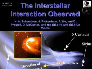
The Interstellar Interaction Observed N. A. Schwadron, J. Richardson, P. Wu, and C. Prested, D. McComas, and the IBEX-Hi and IBEX-Lo Teams Jan 7, 2009
Outline • What we have learned about heliospheric asymmetries and energy distributions • Implications for Models of ENAs • Some Necessary Complications • 100 AU to 1 AU • Response Functions of the Sensors
Interstellar Interaction Components • Outflowing solar wind contributes vast majority of Ram Pressure • Time-dependence through Merged Interaction Regions and Solar Cycle and longer term variations • Heliospheric Magnetic Field (Heliospheric Falts?) • The Local Interstellar Cloud • Inflowing neutral atoms give rise to a hydrogen wall • Pickup Ions Carried Out By the Solar Wind (leading to ACRs) • Interstellar Magnetic Field • Energetic Particles • Galactic Cosmic Rays • Anomalous Cosmic Rays • Suprathermal Tails • Dust, Grains • From interstellar medium • Kuiper Belt grains • Outer Source for Pickup Ions (heavy composition) Courtesy Muller et a, 2006l
Where is the Nose? • Predominantly a mix of H, He, O (neutral and singly ionized particles, GCRs and dust • High FIP neutrals penetrate deeply into the heliosphere (observed as neutrals and Pickup ions) • Gravitational focusing (radiation press. Negligible) • He neutral atoms measureed directly (Ulysses) and from Pickup Ions provide our best mesaurement of interstellar flow direction (Witte et al., 1992, 2004; Moebius 2004, Gloeckler et al, 1996) • Velocity = 26.3 0.4 km/s • T = 6300 340 K • Ec. Long.(J2000) = 75.4 0.5 • Ec. Lat. = 5.1 0.2 • n = 0.015 0.002
Evidence of N/S Asymmetry from H • Interstellar H observed • Ly- • Pickup ions • Inferences from Mass Loading • H experiences significant interaction (charge-exchange) in the heliosheath • inflow speed ~20 km/s, 6 km/s less than He, and higher 1600 K temp (Lallement et al., 1993) • SOHO/SWAN indicates flow deflection by ~4 (Lallement et al., 2005) • Filtration in the heliosheath lowers the density relative to the interstellar medium • LISM H - Nint~0.20.03 cm-3 • Filtered H - Nfilt~0.1 cm-3 Latitude Lallement et al., 2005 Longitude
Asymmetry due to the Interstellar Magnetic Field(?) • Field strength thought to be ~1 G; upper limit 2-4 G • Deflection of H observed by SOH/SWAN suggests effect of asymmetric interstellar magnetic
Voyager 1 Unveils the Heliosheath • The Source of Anomalous Cosmic Rays Missing from near the nose of the termination shock
Effects of a Blunt Termination Shock • Acceleration of ACRs requires ~ 1 year (Mewaldt et al., 1996) • This timescale is similar to that of the motions of field lines from the nose back to the flanks and tail of the termination shock • But recent simulations (e.g., Pogorelov et al., 2006,8) show a more symmetric TS due to neutral interactions
V2 crosses the TS In Aug. 2007 at 84 AU V • Speed decrease starts 82 days, 0.7 AU before TS (but TS is likely moving outward). • Crossing clear in plasma data • Flow deflected as expected • Crossing was at 84 AU, 10 AU closer than at V1
Pickup Ions Carry Substantial Energy • Purpose of shock is to make flow subsonic • BUT, flow remains supersonic wrt thermal plasma in heliosheath. • Energy must reside in pickup ions. Pickup ion energy must be 6-10 keV TS
Decreasing Solar Wind Ram Pressure • Solar wind Ram Pressure decreasing with time • At least part of the reason for the differences in TS location observed by V1/V2 • Solar wind Ram Pressure, Energy, Density Correlated with Magnetic Flux (Schwadron and McComas, 2003, 2006, 2008) Time
How Big a Change in Ram Pressure between V1/V2 Crossings • V1 Crosses Dec, 2004 at 94 • V2 Crosses Aug, 2007 at 84 AU • Dynamic Pressure Changes in Fast Wind ~30% • Dynamic Pressure Changes in Slow Wind much smaller McComas et al., 2008 Note ~1 year lag
N/S Asymmetry Reflected by V1-V2 Differences • Models of TS (e.g., Pogorelov et al, 2006, Opher et al., 2006, 2007) generally show V2 closer than V1 by ~ 10 AU at a given time • The distance observed by V1-V2 difference reflects, in part, a real N/S asymmetry Richardson et al., 2006
Summary of Observational Evidence • Where’s the nose? • He neutral observations (Ulysses) give us our main sense of direction • Nose/Tail Asymmetry • Predicted from Models • Possible Evidence for Blunt Termination Shock from Absence of ACRs near Nose • Overall bluntness debated -- new models including neutral interactions show more spherical shock • North/South Asymmetry • Ly- observations suggest N/S asymmetry, possibly due to asymmetry in interstellar B • V1-V2 difference in TS location also suggests this asymmetry • Heliosheatht thicker in the North • Voyager 2 seems to show dominance of the pickup ion energy • More consistent with the Gruntman et al (2001) weak shock limit
How does it Look in ENAs? Kappa Dist. Opher Model Kappa Dist. Pogorelov Model Maxwellian, Opher Model 0.45 keV 1.1 keV 2.6 keV
Possible N/S Asymmetry Near the Nose • ENA flux at 6.8 keV from Opher et. al’s (2006,2007) MHD model of the heliosheath plasma • Kappa distribution is used with kappa = 2.67
Forward Modeling • Acounts for: • Loss by ionization • Deflection by rad pressure • Energy change through heliospheric transmission • Sensor response functions • Geometric Factors • Angular Response • Energy Response
Global Forward Mapping • Above 0.1 keV, the global symmetries of the heliosphere are preserved in ENA maps • Reduction in magnitude due to ENA ionization-loss
Energy Spectra in Strong and Weak limits • ENA energy spectra provide direct measures of ions beyond TS: • Solar wind • Pickup Protons • Energetic protons • Spectra as a function of direction show 3D configuration of the shock and energy partition of the ions at the shock • Spectra also provide information about how EP pressure modifies the TS and what types of injection processes may be at work there Predicted ENA distributions near HSp nose for strong (black) and weak (green) TS [Gruntman et al., 2001]. ENAs >1 keV are accelerated inner heliosheath protons based on projecting observed distributions beyond TS.
Energy Distribution Mapping • Energy dependent .. • ENA ionization loss • ENA deflection • These effects are all stronger at low energies
Incident Flux at 1 AU • We have 14 channels: {hide-1 .. hide-6, lode-1 .. lode-8} • We have one (H) differential energy flux j(E) (O is later) • The channels are coupled through the sensor response:
Orbit-Spin Frame • The natural frame to work in for all of the above is a frame built around IBEX's mean spin for the orbit. • For Direct Events the sky is well sampled in the spinward direction (α) • No information in the transverse direction (β) • Our collimators are narrow enough that the effects are negligible for the moment. (A 1D FFT can be used if desired.)
Follow Trajectory out to 100 AU • Trajectory can be traced backwards • This can be as simple or as complicated as you chose to make it • Simplest central-force, constant-μ used here • Can be easily made more sophisticated • Survivability is important • Deflection angle changes with energy
Collecting Multiple Orbits • Combining orbits can be done in any frame--- used an ecliptic one here • Exaggerated the deflection (δ) for two orbits that are weeks apart • The flux from pixels at 1 AU will contribute to one or more pixels at 100 AU. • Different part of the band refer to different HS energies (E)
Summary • We are about to discover a new global view of the heliosphere from ENAs! • We expect to see asymmetries • Nose/Tail asymmetry (which one should be brighter, we don’t yet know) • North/South asymmetry (perhaps). Brighter emissions from the North? • The energy distribution • Voyager 2 results suggest prominence of pickup ions • Will we see a knee in the pickup ions • Relative contribution of kappa function & pickup-like distribution? • Model interface at the IBEX Science Operations Center • A first version up and running • Forward modeling interfaces to models (to be expanded as much as possible/desired) • Reverse modeling account for heliospheric transmission effects
View time per Pixel for 2 year Mission Reduction in view time due to magnetosphere obscuration
Gravitational Focusing and the H shadow Primary component from itnerstellar flow • Backscattered Ly- (Bertaux and Blamont,1971; Thomas and Krassa, 1971) and He 58.4 nm radiation (Weller and Meier, 1979) reveal radiation pressure at work • Radiation pressure weak for He, gravitational focusing cone • Radiation pressure comparable to gravity for H, interstellar H shadow Secondary component from interaction
The Effects of Dust • Grains serve as a secondary source of pickup ions • Inner & outer source • Pickup Ions accelerated into Low-FIP ACRs