Download
1 / 17
180 likes | 325 Views
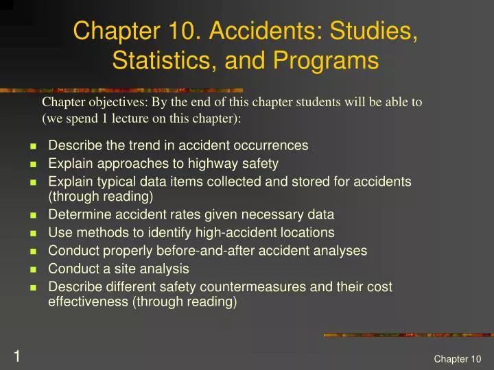
Chapter 10. Accidents: Studies, Statistics, and Programs. Chapter objectives: By the end of this chapter students will be able to (we spend 1 lecture on this chapter):. Describe the trend in accident occurrences Explain approaches to highway safety

E N D
Chapter 10. Accidents: Studies, Statistics, and Programs Chapter objectives: By the end of this chapter students will be able to (we spend 1 lecture on this chapter): • Describe the trend in accident occurrences • Explain approaches to highway safety • Explain typical data items collected and stored for accidents (through reading) • Determine accident rates given necessary data • Use methods to identify high-accident locations • Conduct properly before-and-after accident analyses • Conduct a site analysis • Describe different safety countermeasures and their cost effectiveness (through reading) Chapter 10
10.1 Introduction Fatality rates are decreasing but the number of fatalities has plateaued. Check: http://www.fhwa.dot.gov/policyinformation/statistics/2007/ and www-fars.nhtsa.dot.gov/ Chapter 10
10.2 Approaches to highway safety (Page 239-242) Chapter 10
Type of Safety Belt Use Laws, by State: As of 2000 Latest Info about Seat Belt Law Chapter 10
10.3 Accident data collection and record systems • One of the most basic functions of traffic engineering is keeping track of the physical inventory. Collision diagram Accident spot map Chapter 10 Example: AIMS (Accident Info Mgmt System) by JMW Engineering
10.4 Accident statistics • Types of accidents • Numbers of accidents Occurrence • No. of deaths • No. of injuries • Categories of vehicles • Categories of drivers Types of statistics Involvement Severity http://www-nrd.nhtsa.dot.gov/departments/nrd-30/ncsa/STSI/49_UT/2008/49_UT_2008.htm/ Chapter 10
Typical accident rates used “Bases” are needed to compare the occurrence of accidents at different sites. • Population based: • Area population (25 deaths per 100,000 pop) • No. of registered vehicles (7.5 deaths per 10,000 registered vehicles) • No. of licensed drivers (5.0 deaths per 10,000 licensed drivers) • Highway mileage (5.0 deaths per 1,000 miles) • Exposure based: • VMT (5.0 deaths per 100 million VMT) • VHT (5.0 deaths per 100 million VHT) Severity index: No. of deaths/accident (0.0285 death per accident) No. of injuries/accident • Typical basic accident rates: • general accident rates describing total accident occurrence • fatality rates describing accident severity • involvement rates describing the types of vehicles and drivers involved in accidents Chapter 10
Types of statistical displays The purpose of the display dictates the type of display – temporal, spatial, accident type, etc. Chapter 10
5% z = 1.645 Determining high-accident locations (p.251) H0: Accident rate at the location under consideration in the group is equal to the average rate of the group. H1: Accident rate at the location under consideration in the group is higher than the average rate of the group. This is a one-tailed test. Why? Example: Highway Section 33 has 210 accident/100MVMT. The mean accident rate for the similar classification group = 89 accidents/100MVMT, SD = 64 accidents/100MVMT. Should an analyst flag Section 33 as hazardous? With the 95% confidence level? Locations with a higher accident rate than this value would normally be selected for specific study. Chapter 10
Determining high-accident locations: Expected value analysis (from Garber & Hoel) • Note this method is used only to compare sites with similar characteristics. H0: Accident rate at the location under consideration in the group is equal to the average rate of the group. H1: Accident rate at the location under consideration in the group is not equal to the average rate of the group (In another words, we are trying to find whether the site under study is “unusual” or not. We are not specifically proving it is “over-represented” or not.) z = 1.96 for the 95% confidence level Locations with a higher accident rate than this value would normally be selected for specific study. Not over-represented or under-represented “Under-represented” “Over-represented” Chapter 10
Example: An intersection with 14 rear-end, 10 LT, and 2 right-angle collisions for 3 consecutive years • Check about rear-end collisions Rear-end collisions are over-represented at the study site at 95% confidence level, since 14 > 10.34. • Check about LT collisions LT collisions are not over-represented or under-represented at the study site at 95% confidence level, since 0.88<10 < 12.92. • Check about right-angle collisions Right-angle collisions are under-represented at the study site at 95% confidence level, since 2 < 2.4. Chapter 10
10.4.5 Statistical analysis of before-after accident data Method 1: Use the Normal Approximation method: z1 = test statistic, 1.96 at the 95% confidence level for a “change”, 1.645 for a “reduction.” fA = No. of accidents in the “after” study fB = No. of accidents in the “before” study Assumption: Accident occurrence is random (Poisson distribution) Mean and variancehave the same value if the sample follows the Poisson distribution (eq 7-15, p.144). When two samples are combined the variances are added. It is assumed the difference in the before and after occurrence is normally distributed. (Accident occurrence itself is Poisson distributed.) This method is however not listed in the current Manual of Transportation Engineering Studies. Chapter 10
Statistical analysis of before-after accident data (cont) Method 2: The Modified Binomial Test Example: Before 14 conflicts were observed at a stop-sign controlled intersection. After the installation of a signal, they observed 7 conflicts. Were the signal effective? Solution: Figure on the right shows that for 14 before conflicts you need a 60% reduction to be significant at the 95% CL. 7/14=50% reduction. So, you cannot reject the null hypothesis (i.e., before = after). Statistically no effect by the signal. Chapter 10
10.5 Site analysis • Purposes: • Identify contributing causes • Develop site specific improvements • Two types of info: • Accident data • Environment & physical condition data The first thing you do is visit the site and prepare a condition diagram of the site. Chapter 10
Site analysis (cont) Then we prepare a collision diagram. Chapter 10
Site analysis (cont) Group accidents by type and answer the following 3 questions, which will lead you to possible countermeasures. • What drivers actions lead to the occurrence of such an accident? • What conditions existing at the location could contribute toward drivers taking such actions • What changes can be made to reduce the chance of such actions occurring in the future? Rear-end collisions: Driver: Sudden stop & Tailgating Environment: Too many accesses and interactions with vehicles in/out of the accesses, bad sight distance, short/long yellow interval, inappropriate location of stop lines, etc. (Table 10-4 is useful for this task) Chapter 10
10.6 Development of countermeasures • See Table 10.3 Illustrative programmatic safety approaches. • Table 10.4 Illustrative site-specific accident countermeasures. Chapter 10