Download
1 / 49
500 likes | 684 Views
Computational Gene Finding. Greg Voronin Hui Zhao Xueyi(Judy) Xiao. CIS786 Intro to Comp Biol Instructor: Dr. Barry Cohen. The Challenge. Presented By Greg Voronin. Generate predictions of gene locations from primary genomic sequence by computational means Two principle means:

E N D
Computational Gene Finding Greg Voronin Hui Zhao Xueyi(Judy) Xiao CIS786 Intro to Comp Biol Instructor: Dr. Barry Cohen
The Challenge Presented By Greg Voronin • Generate predictions of gene locations from primary genomic sequence by computational means • Two principle means: • Database searching • Statistical Methods
The Computational Model • Representing the biology in a framework amenable to mathematical/statistical methods • Exon classification, sequence features, signal profiles • What is an exon and what properties does the sequence of an exon hold? • How is an exon recognized and processed?
The Nature of The Data • What is the primary genomic sequence? • “Nor is the available sequence a single continuous and exact sequence for each chromosome… [ the HGP ] is represented by a set of sequences that cover the genome is a statistical sense but have a very large number of gaps.” • Many genes are as large or larger than the contigs in the HGP • Finding genes will depend on the accuracy of the scaffold of their contigs
Back to Beginning • What is a gene? • A biological model, a mathematical model and computational representation • The programs we evaluate take these factors into account in their underlying model
MZEF • Michael Zhang’s Exon Finder • Utilizes quadratic discriminant analysis (QDA) to classify sequence into gene and non-gene groups • QDA is a multivariate statistical pattern recognition method • “Draws” a curved boundary between groups of different classes
Key Elements of QDA • Entities are represented by an n-dimensional vector of feature values • Two classes of entities are categorized by their respective multinormal distribution • Each class has its own mean vector • The mean of each feature • An appropriate distance function is central to the calculation of the posterior probabillity of group membership of a given unknown entity given its specific feature vector.
Mahalanobis Distance • The actual posterior probabillity function is more complex, but this is the distance component: • ( x – mi )T Si-1 ( x – mi )
MZEF Specifics • MZEF uses the following features: • Exon length, exon-intron transition, branch site score, 3’ss score, exon score, strand score, frame score, 5’ss score, intron-exon transition • 9 dimensional feature vector • Training sets of known exons and “non-exons” are used to establish the class characterisitics • Supervised learning
…GATC… to Gene Cells recognize genes from DNA sequence. Can we?? The Hidden Markov Model Method HMMgene Presented By Hui Zhao
HMMs are Statistical Models • Definition: • Any mathematical construct that attempts to parameterize a random process • Example: A normal distribution • Assumptions • Parameters • Estimation • Usage • HMMs are just a little more complicated…
Primary HMM Assumptions • Observations are ordered • Random processes can be represented by a stochastic finite state machine with emitting states • transition probabilities and emission probabilities.
How do we find the model probabilities? • This is called training • We start with an architecture and a set of observed sequences • The training process iteratively alters its parameters to fit the training set • The trained model will assign the training sequences high probability – but can it generalize?
HMM Usage – two major tasks • Evaluate the probability of an observed sequence given the model (Forward) • Find the most likely path through the model for a given observation sequence (Viterbi)
Gene Finding: An Ideal HMM Application • Our Objective: • To find the coding and non-coding regions of an unlabeled string of DNA nucleotides • Our Motivation: • Assist in the annotation of genomic data produced by genome sequencing methods • Gain insight into the mechanisms involved in transcription, splicing and other processes
Why HMMs might be a good fit for Gene Finding • The observations within a sequence are ordered • A DNA sequence is a set of ordered observations • Designing the architecture is straight forward: • Easy to measure success • Training data is available from various genome annotation projects
A HMM genefinder • States represent standard gene features: intergenic region, exon, intron, perhaps more (promotor, 5’UTR, 3’UTR, Poly-A,..). • Observationsare things like state-dependent base composition. • In a HMM, length of each statemust be included as well. • Finally, reading frames and both strands must be dealt with.
3’ Several problems can occur 5’ correct gene structure extended exon missing exon additional exon missing intron extended gene model
Predicts whole genes in any given stretch of DNA • Uses Hidden Markov Models (HMM) to maximize probability of accurate prediction • This allows confidence levels to be determined and "Best Prediction" as well as potential alternative splicing predictions • Outputs splice sites, start and stop codons, alternative predictions • Trained for human and C. elegans HMMgene Krogh (1997) In Proc. 5th Conf. Intel. Sys. Mol Biol. pp179-186
HMMGene • Uses an extended HMM called a CHMM • CHMM = HMM with classes • Takes full advantage of being able to modify the statistical algorithms • Uses high-order states • Trains everything at once
e.g: P(G, I | A,C,G,G,T) P(G, E | A,C,G,G,T) How does HMMGene work? 1) 5th order HMM assumes: P(xi | xi-1,xi-2, xi-3, xi-4, xi-5) is different in Introns, Exons, etc.. 2) Construct the model
3) In a CHMM states emit a pair 2. How does HMMGene work? 4) Use Viterbi (n-best) to find a path through the CHMM = a labeled gene 5) Use the forward algorithm to measure P(gene | model) –using n-best.
A DNA sequence containing one gene. For each nucleotide its label is written below. The coding regions are labeled ‘C’, the introns ‘I’, and the intergenic regions ‘0’. HMMGene calls these class labels in a CHMM.
HMMGene • Does not use the standard ML method which optimizes the probability of the observed sequence – instead it maximizes the probability of the correct prediction. • Only one conference paper describes the algorithm. There is a web site to run the algorithm, and it's performance has been compared to other algorithms. • No complete description of the algorithm is available – in the 1997 paper the author states "… the details of HMMGene will be described elsewhere (in prep)" – but unfortunately the detailed paper has not been published.
P(x) P(y) … HMMgene and HMM Disadvantages • Markov Chains • States should be independent • P(y) must be independent of P(x) -usually not true • Local maxima • Model may not converge the optimal parameter set • Over-fitting • More training is not always good-set may be too small
Summary • HMMgene finds whole genes in anonymous DNA with correctly spliced exons. • It can predict several whole or partial genes in one sequence. • If some features of a sequence are known, such as hits to ESTs, proteins, or repeat elements, these regions can be locked as coding or non-coding and then the program will find the best gene structure under these constraints.
GENSCAN (v1.0) Presented By Xueyi (Judy) Xiao • A computer program identifying complete exon & intronstructures of genes ingenomic DNA. • Developed by Chris Burge (Burge 1997), in the research group of Samuel Karlin, Dept of Mathematics, Stanford Univ. • Original server @Stanford New server @MIT (seq_len <= 500 kb); Servers are also maintained by the Pasteur Institute, Paris and by the GENSCAN web server at DKFZ/EMBnet, Heidelberg • Implementations • web serverhttp://genes.mit.edu/GENSCAN.html • email serverhttp://genes.mit.edu/GENSCANM.html • local copy downloaded under a license agreement
How does It Work? • Designed to predict complete gene structures • Introns and exons • Promoter sites • Polyadenylation signals • Larger predictive scope • Partial and Complete genes • Multiple genes separated by intergenic DNA in a seq • Consistent sets of genes on either/both DNA strands • Not use similarity-based methods • Based on a general probabilistic modelof genomic sequences composition and gene structure
Model of Genomic Sequence Structure Fig. 3, Burge and Karlin 1997
Graphic View Optimal Exon Suboptimal Exon Initial Exon Internal Exon Terminal Exon Single-Exon gene
Is It Good? • Accuracy: Substantiallyhigher accuracies whentested on standardized sets of human & vertebrategenes, with 75-80% of exons identifiedexactly. • Reliability: Able to indicate fairly accuratelythereliability of each predicted exon. • Consistency: Consistentlyhigh levels of accuracy, forseqsof differing C+G content and fordistinct groups ofvertebrates.
Why not Perfect? • Gene Number usually approximately correct, but may not • Organism primarily for human/vertebrate seqs; maybe lower accuracy for non-vertebrates. ‘Glimmer’ & ‘GeneMark’ for prokaryotic or yeast seqs • Exon and Feature Type Internal exons > Initial or Terminal exons; Exons > Polyadenylation or Promoter signals(‘NNPP’) • Biases in Test Set The Burset/Guigó (1996) dataset: • toward short genes with relatively simple exon/intron structure The Rogic (2001) dataset: • DNA seqs: GenBank r-111.0 (04/1999 <- 08/1997); • source organism specified; • consider genomic seqs containing exactly one gene; • seqs>200kb were discarded; mRNA seqs and seqs containing pseudo genes or alternatively spliced genes were excluded.
What are They doing NOW? The research group @MIT is currently developing another program, GenomeScan, which is more accurate when a moderate or closely related protein seq is available.
TEST OF METHODS • Sample Tests reported by Literature • Test on the set of 570 vertebrate gene seqs (Burset&Guigo 1996) as a standard for comparison of gene finding methods. • Test on the set of 195 seqs of human, mouse or rat origin (named HMR195) (Rogic 2001). • Self-Test done by our group • Dataset: Intron-less(Single-exon), -rich(Multi-exon), -poor(Random) • Organism: Human • Methods: all of the three • Steps
Where to get the dataset for Self-Test? http://www.ncbi.nlm.nih.gov/genome/guide/human/
TP FP TN FN TP FN TN Actual Predicted Actual Coding / No Coding TP FP Predicted No Coding / Coding FN TN Accuracy Measures Sensitivity vs. Specificity(adapted from Burset&Guigo 1996)
Results:Accuracy Statistics Table: Relative Performance(adapted & added from Rogic 2001) # of seqs - number of seqs effectively analyzed by each program; in parentheses is the number of seqs where the absence of gene was predicted; Sn -nucleotide level sensitivity; Sp - nucleotide level specificity; CC - correlation coefficient; ESn - exon level sensitivity; ESp - exon level specificity
Testing ‘Random’ Sequences Presented By Greg Voronin • These gene finding programs model statistical trends and properties • Can they be fooled by ‘random’ sequences • Generate a preliminary measure of accuracy • Java program written to generate ‘random’ sequences of a,t,g,c • 3 groups of sequences 5k, 10k & 30K • Sent to BLAST then GeneMachine
Testing Results • BLAST: bit score E-value • 5k 42 5.7 • 10k 44 3.0 • 30k 42 8.7 • GeneMachine: 5k 10k 30K • MZEF 1 5 14 • GenScan 3 11 26 • HMMgene 7 11 42
New directions Presented By Hui Zhao • Computational Gene Finding has rapidly evolved since it started 20 years ago. • The advent of full-length genomic sequences has provided data and increased the requirements. • Gene annotation has direct medical implications on the design of pharmaceuticals and the understanding of the genetic component of diseases. • Gene finding remains largely an unsolved problem.
New directions • The growing quantities of training data for the models should improve their performance. • Algorithms that combine the inputs from several models in a weighted voting scheme should be considered to try to get the best from all of the methods. • Many other AI approaches can be used to meet this challenge including decision trees, neural networks and rule-based systems
Challenges and Discoveries Ahead • Eukaryotic gene finding continues to be an active and important area – more research is required into algorithms with greater accuracy • Expertise in computational biology is also required – which means training in both: computer science and molecular biology • More classes like this…