Download
1 / 33
330 likes | 559 Views
The Calibration Process. Calibration of a flow model refers to a demonstration that the model is capable of producing field-measured heads and flows which are the calibration values.

E N D
The Calibration Process • Calibration of a flow model refers to a demonstration that the model is capable of producing field-measured heads and flows which are the calibration values. • Calibration is accomplished by finding a set of parameters, boundary conditions, and stresses that produce simulated heads and fluxes that match field-measured values within a pre-established range of error.
Targets in Model Calibration • Head measured in an observation well is known as a target. Baseflow measurements or other fluxes are also used as targets during calibration. • The simulated head at a node representing an observation well is compared with the measured head in the well. (Similarly for flux targets…) • Residual error = observed - simulated • During model calibration, parameter values (e.g., R and T) are adjusted until the simulated head matches the observed value within some acceptable range of error. Hence, model calibration solves the inverse problem.
Inverse Problem • Objective is to determine values of the parameters and hydrologic stresses from information about heads, whereas in the forward problem system parameters such as hydraulic conductivity, specific storage, and hydrologic stresses such as recharge rate are specified and the model calculates heads. • The inverse problem is an estimation of boundary conditions, hydrologic stresses, and the spatial distribution of parameters by methods that do not involve consideration of heads.
Calibration can be performed: • steady-state • Requires some flux input to the system • transient data sets.
Information needed for calibration: • head values and fluxes or other calibration data (called sample information), • parameter estimates (called prior information) that will be used during the calibration process.
Sample Information • Heads • Sources of error • transient effects that are not represented in the model. • measurement error associated with the accuracy of the water level measuring device • Interpolation Error • Calibration values ideally should coincide with nodes, but in practice this will seldom be possible. This introduces interpolation errors caused by estimating nodal head values. This type of error may be 10 feet or more in regional models. The points for which calibration values are available should be shown on a map to illustrate the locations of the calibration points relative to the nodes. Ideally, heads and fluxes should be measured at a large number of locations, uniformly distributed over the modeled region.
Examples of Sources of Error • Surveying errors • Errors in measuring water levels • Interpolation error • Transient effects • Scaling effects • Unmodeled heterogeneities
Sample Information • Fluxes • Field-measured fluxes, such as baseflow, springflow, infiltration from a losing stream, or evapotranspiration from the water table may also be selected as calibration values. • associated errors for flux are usually larger than errors associated with head measurements. • Calibration to flows gives an independent check on hydraulic conductivity values.
Prior Information • Calibration is difficult because values for aquifer parameters and hydrologic stresses are typically known at only a few nodes and, even then, estimates are influenced by uncertainty. • Prior information on hydraulic conductivity and/or transmissivity and storage parameters is usually derived from aquifer tests. • Prior information on discharge from the aquifer may be available from field measurements of springflow or baseflow. • Direct field measurements of recharge are usually not available but it may be possible to identify a plausible range of values. • Uncertainty associated with estimates of aquifer parameters and boundary conditions must also be evaluated.
Calibration Techniques • two ways of finding model parameters to achieve calibration • (1) manual trial-and-error adjustment of parameters • (2) automated parameter estimation. • Manual trial-and-error calibration was the first technique to be used and is still the technique preferred by most practitioners.
Calibration parametersare parameters whose values are uncertain. Values for these parameters are adjusted during model calibration. Typical calibration parameters include hydraulic conductivity and recharge rate. Parameter values can be adjusted manually by trial and error. This requires the user to do multiple runs of the model. …or parameter adjustment can be done with the help of an inverse code.
Trial-and-Error Calibration • Parameter values assigned to each node or element in the grid. • The values are adjusted in sequential model runs to match simulated heads and flows to the calibration targets. • For each parameter an uncertainty value is quantified. Some parameters may be known with a high degree of certainty and therefore should be modified only slightly or not at all during calibration. • The results of each model execution are compared to the calibration targets; adjustments are made to all or selected parameters and/or boundary conditions, and another trial calibration is initiated. • 10s to 100s of model runs may be needed to achieve calibration. • No information on the degree of uncertainty in the final parameter selection • Does not guarantee the statistically best solution, may produce nonunique solutions when different combinations of parameters yield essentially the same head distribution.
Automated Calibration • Automated inverse modeling is performed using specially developed codes • Example PEST – Parameter ESTimation, • Direct solution - unknown parameters are treated as dependent variables in the governing equation and heads are treated as independent variables. • The direct approach is similar to the trial-and-error calibration in that the forward problem is solved repeatedly. However, the code automatically checks and updates the parameters to obtain the best solution. • The inverse code will automatically find a set of parameters that matches the observed head values. • An automated statistically based solution quantifies the uncertainty in parameter estimates and gives the statistically most appropriate solution for the given input parameters provided it is based on an appropriate statistical model of errors.
Evaluating the Calibration • The results of the calibration should be evaluated both qualitatively and quantitatively. Even in a quantitative evaluation, however, the judgment of when the fit between model and reality is good enough is a subjective one. • There is no standard protocol for evaluating the calibration process. • Traditional measures of calibration • Comparison between contour maps of measured and simulated heads • A scatterplot of measured against simulated heads is another way of showing the calibrated fit. Deviation of points from the straight line should be randomly distributed.
Perfect fit Basecase simulation for the Final Project
Expressing differences between simulated and measured heads • The mean error (ME) is the mean difference between measured heads (hm) and simulated heads (hs). • where n is the number of calibration values. • Simple to calculate • Both negative and positive differences are incorporated in the mean and may cancel out the error. • Hence, a small mean error may not indicate a good calibration.
Expressing differences between simulated and measured heads • The mean absolute error (MAE) is the mean of the absolute value of the differences in measured and simulated heads. • All errors are positive. • Hence, a small mean error may would indicate a good calibration.
Expressing differences between simulated and measured heads • The root mean squared (RMS) error or the standard deviation is the average of the squared differences in measured and simulated heads. • As with MAE, all errors are positive. • Hence, a small mean error may would indicate a good calibration.
The RMS is usually thought to be the best measure of error if errors are normally distributed. However, ME and MAE may provide better error measures (Figure 32).
Sensitivity Analysis • Purpose: to quantify the uncertainty in the calibrated model caused by uncertainty in the estimates of aquifer parameters, stresses, and boundary conditions. • Process: Calibrated values for hydraulic conductivity, storage parameters, recharge, and boundary conditions are systematically changed within the previously established plausible range. The magnitude of change in heads from the calibrated solution is a measure of the sensitivity of the solution to that particular parameter. • Sensitivity analysis is typically performed by changing one parameter value at a time. • A sensitivity analysis may also test the effect of changes in parameter values on something other than head, such as discharge or leakage