Download
1 / 41
410 likes | 415 Views
Linear Filters in StreamIt. Andrew A. Lamb MIT Laboratory for Computer Science Computer Architecture Group 8/29/2002. Outline. Introduction Dataflow Analysis Hierarchal Matrix Combinations Performance Optimizations. Basic Idea. Filter A a=pop(); b=pop(); c=(a+b)/2 + 1; push(c);.

E N D
Linear Filters in StreamIt Andrew A. Lamb MIT Laboratory for Computer Science Computer Architecture Group 8/29/2002
Outline • Introduction • Dataflow Analysis • Hierarchal Matrix Combinations • Performance Optimizations
Basic Idea Filter A a=pop(); b=pop(); c=(a+b)/2 + 1; push(c); Matrix Mult. x y y =xA+ b
What is a Linear Filter? • Generic filters calculate some outputs (possibly) based on their inputs. • Linear filters: outputs (yj) are weighted sums of the inputs (xi) plus a constant. for b constant wi constant for all i N is the number of inputs
Linearity and Matricies • Matrix multiply is exactly weighted sum • We treat inputs (xi) and outputs (yj) as vectors of values (x, and y respectively) • Filter is represented as a matrix of weights A and a vector of constants b • Therefore, filter represents the equation y = xA + b
Usefulness of Linearity • Not all filters compute linear functions • push(pop()*pop()); • Many fundamental DSP filters do • DFT/FFT • DCT • Convolution/FIR • Matrix Multiply
Example: DFT Matrix DFT: row n column m
Example: IDFT Matrix IDFT: row m column n
Usefullness, cont. • Matrix representations • Are “embarrassingly parallel” 1 • Expose redundant computation • Let us take advantage of existing work in DSP field • Well understood mathematics 1: Thank you, Bill Thies
Outline • Introduction • Dataflow Analysis • Hierarchal Matrix Combinations • Performance Optimizations
Dataflow Analysis • Basic idea: convert the general code of a filter’s work function into an affine representation (eg y=xA+b) • The A matrix represents the linear combination of inputs used to calculate each output. • The vector b represents a constant offset that is added to the combination.
“Linear” Dataflow Analysis • Much like standard constant prop. • Goal: Have a vector of weights and a constant that represents the argument to each push statement which become a column in A and an entry in b. • Keep mappings from variables to their linear forms (eg vector + constant).
“Linear” Dataflow Analysis • Of course, we need the appropriate generating cases, eg • constants • pop/peek(x)
“Linear” Dataflow Analysis • Like const prop, confluence operator is set union. • Need combination rules to handle things like multiplication and addition (vector add and constant scale)
Ridiculous Example a=peek(2); b=pop(); c=pop(); pop(); d=a+2b; e=d+5;
Ridiculous Example a a=peek(2); b=pop(); c=pop(); pop(); d=a+2b; e=d+5;
Ridiculous Example a a=peek(2); b=pop(); c=pop(); pop(); d=a+2b; e=d+5; b
Ridiculous Example a a=peek(2); b=pop(); c=pop(); pop(); d=a+2b; e=d+5; b c
Ridiculous Example a a=peek(2); b=pop(); c=pop(); pop(); d=a+2b; e=d+5; b c d
Ridiculous Example a a=peek(2); b=pop(); c=pop(); pop(); d=a+2b; e=d+5; b c d e
Constructing matrix A Filter A: a filter code b push(b); push(a);
Constructing matrix A Filter A: a filter code b push(b); push(a);
Constructing matrix A Filter A: a filter code b push(b); push(a);
Big Picture FIR Filter weights1 = {1,2,3}; weights2 = {4,5,6}; float sum1 = 0; float sum2 = 0; float mean1 = 5; mean2 = 17; for (int i=0; i<3; i++) { sum1 += weights1[i]*peek(3-i-1); sum1 += weights1[i]*peek(3-i-1); } push(sum2 – mean2); push(sum1 – mean1); pop(); push = 2 pop = 1 peek = 3
Big Picture, cont. Matrix Mult. x y y =xA+ b size(x) = 3 size(y) = 2
Outline • Introduction • Dataflow Analysis • Hierarchal Matrix Combinations • Performance Optimizations
Combining Filters • Basic idea: combine pipelines, splitjoins (and possibly feedback loops) of linear filters together • End up with a single large matrix representation • The details are tricky in the general case (eg I am still working on them)
Combining Pipelines The matrix C is calculated as A’B’ where A’ and B’ have been appropriately scaled and duplicated to make the dimensions work out. In the case where peek(B) pop(B), we might have to use two stage filters or duplicate some work to get the dimensions to work out. [A] [B] ye olde pipeline [C] single filter
Combining Split Joins [A1] [A2] splitter joiner [C] [A3] [AN] single filter ye olde SplitJoin A split join reorders data, so the columns of C are interleaved copies of the columns of A1 through AN. Matching the rates of A1 through AN is a challenge that I am still working out.
Combining Feedback Loops joiner splitter [A] ? [B] ye olde FeedbackLoop It is unclear if we can do anything of use with a FeedbackLoop construct. Eigen values might give information about stability, but it is not clear if that is useful… more thought is needed.
Outline • Introduction • Dataflow Analysis • Hierarchal Matrix Combinations • Performance Optimizations
Performance Optimizations • Take advantage of our compile time knowledge of the matrix coefficients. • eg don’t waste computation on zeros • Try and leverage existing DSP work on factoring matricies. • Try to recognize parallel structures in our matrices. • Use frequency analysis.
Factoring for Performance 16 multiplies 12 adds 14 multiplies 6 adds
SPL/SPIRAL • Software package that will attempt to find a fast implementation signal processing algorithms described as matrices. • It attempts to find a sparse factorization of an arbitrary matrix. • It can automatically derive FFT (eg the Cooley-Turkey algorithm) from DFT definition. • Claim that their performance is FFTW1. 1. See http://www.fftw.org
Recognize Parallel Structure • We can go from SplitJoin to matrix. • Perhaps we can recognize the reverse transformation. • Also, implement blocked matrix multiply to keep parallel resources busy.
Frequency Analysis Instead of computing the matrix product straight up, possibly go to frequency domain. Rids us of offset vector (added to response at f=0). Might allow additional optimizations (because of possible symmetries exposed in frequency domain). [A] [A’] DFT IDFT
Work left to do • Implementation of single filter analysis. • Combining hierarchical constructs. • Understand the math of automatic matrix factorizations (group theory). • Analyze frequency analysis. • Implement optimizations. • Get results.
Questions for the Future • Are there any other optimizations? • Can we produce inverted matrices • programmer codes up transmitter and StreamIt automatically creates the receiver.1 • How many cycles of a “real” DSP application are spent computing linear functions? • Can we combine the linear description of what happens inside a filter with the SARE representation of what is happening between them? (POPL paper) 1. Thank you, BT