Statistics: an introduction

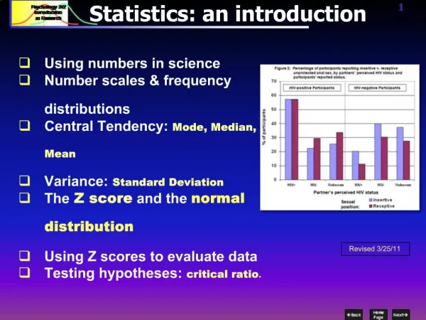
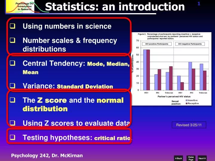
1. Statistics: an introduction • Using numbers in science • Number scales & frequency distributions • Central Tendency: Mode, Median, Mean • Variance: Standard Deviation • The Z score and the normal distribution • Using Z scores to evaluate data • Testing hypotheses: critical ratio. Revised 3/25/11

2. Research questions, hypotheses & designs  • Using numbers in science • Number scales & frequency distributions • Central Tendency: Mode, Median, Mean • Variance: Standard Deviation • The Z score and the normal distribution • Using Z scores to evaluate data • Testing hypotheses: critical ratio.

3. Why Use Numbers in Science? • Comparability of research outcomes • Across groups or conditions within a study • Across studies • Statistical operations • Testing for “statistical significance” • Calculation of effect sizes • Clarity and specificity of measures • Operational definitions!! • Common language (of science, commerce, etc.) Statistics introduction 1

4. Costs and & benefits of numbers Virtues of numerical data: • Representing data by numbers helps clarify and simplify communication • Can show general trend or “common denominator” in the data Danger of numerical data: • Can over-simplify / ignore individual differences • Liable to misrepresentation or manipulation, as per Broder’s article… Statistics introduction 1

5. The danger of reducing complex social processes to simple numbers: A. Theory & hypotheses are more important than numbers • Testing why or how something works is more important than collecting simple numbers. B. Where does the single number come from? • Choice to emphasize one key variable or outcome is often political, not scientific. • Selection of some statistics (i.e., the M in highly skewed data such as income)can be very politically biased (e.g., tax cuts). C. Biased search for confirmatory measure. • Does having a gun in a household increase or decrease safety? • Is ObamaCare “working”? Statistics introduction 1

6. Political (mis)uses of scientific data D. Ambiguity in the interpretation of data: Increased rates autism: shift in actual disorder, or lower threshold for reporting cases? Rising divorce rate: breakdown in family structure, or lower willingness to stay in poor / abusive relationships? E. Simply ignoring disconfirming data: Project DARE continues as a politically favored but ineffective drug abuse prevention program Youth violence and criminal proceedings: see reading by Overholster Statistics introduction 1

7. Thus… • Representing nature in terms of numbers is important to scientific progress • Key for operational definitions • Provide powerful analytic & communication tools • Understanding ANY statistic requires that we understand how it was derived • Statistical statements can be literally / technically “true” but misleading. • What context was the statistic was drawn from? • What else do we need to know to evaluate it? • Political or commercial misuse of numerical / statistical information is common and problematic. There are lies, damned lies, and statistics. -- Mark Twain Statistics introduction 1

8. Some basic terms:  Characteristic or attribute with different levels or qualities (e.g., age, speed, effort, attention). • Variable  One level or state of a variable (e.g., age = 21, ethnicity = Latino). • Value • Distribution  Set of scores (each with its own value) for one variable(e.g., distribution of student ages). • Central Tendency  Primary “drift” of a set of scores (Mean, Mode, or Median).  Measure of how much the scores in a distribution differ from each other. • Variance  Mathematical characteristic of (variable that describes an aspect of…) a population. • Parameter  Mathematical characteristic of a sample. • Statistic Statistics introduction 1

9. Research questions, hypotheses & designs • Using numbers in science • Number scales & frequency distributions • Central Tendency: Mode, Median, Mean • Variance: Standard Deviation • The Z score and the normal distribution • Using Z scores to evaluate data • Testing hypotheses: critical ratio.  Week 3; Experimental designs

10. Types of numerical scales Ratio • Scales of physical properties. Used for physical description: temperature, elapsed time, height Interval Arbitrary or relative ψscales Common in behavioral research, e.g., attitude or rating scales. Ordinal Rank order with non-equal intervals Simple finish place, rank in organization, most, 2nd most, 3rd most... Categorical Categories only Typical of inherent categories: ethnic group, gender, zip code Continuous Scales Statistics introduction 1

11. Scale details Ratio Interval Ordinal Categorical Ratio Scales; temperature, height, blood pressure.. Each scale value describes a physical reality • Batting average: % hits / at bats • The zero point is grounded in a physical property • 0 hits is meaningful • Water always freezes at 32oF • Each scale point is absolute • 32o has an absolute meaning, not just relative to other temperatures. • Each interval is continuous & exactly equal: • 30oF  40oF ≡ 90oF  100oF • Used for correlational designs, or as dependent variable in experiments. Statistics introduction 1

12. Interval scales Ratio Interval Ordinal Categorical • Interval Scales; e.g, attitude rating scale, IQ… • Not grounded in physical reality; “ψ reality” only • Correlational designs, dependent variable in experiments. • Does nothave a “0” point; each scale point is relative • Intervals are designed to be the same… • … but may not be. Does not agree at all Strongly agree 1 2 3 4 5 6 7 = In agreeing with an attitude statement (242 has changed my life…) this is a bigger ψ step than this Statistics introduction 1

13. Interval scales Ratio Interval Ordinal Categorical • Ordinal Scales; e.g., rank order • Also not grounded in physical reality • Relative “strength” or placement on a scale • Primarily correlational / measurement designs. • No “0” point; each scale point is relative • Provides no information about intervals Least preferred Text discus- lecture Instructor sions Most preferred Intervals between each scale point are arbitrary… (Many interval scales may actually be ordinal…) Statistics introduction 1

14. Interval scales Ratio Interval Ordinal Categorical • Categorical Scales • Simple groups / categories • Measurementstudies (e.g., epidemiology) • Independent Variable in an experiment. • Binary (“nominal”) measures: 2 levels only • Experimental v. control group • “Drug user” v. not • Categorical: >2 levels • Ethnic group, City neighborhood, primary drug used… • Groups may be inherent (gender, ethnicity) or arbitrary (experimental group…). Statistics introduction 1

15. Two central ways of using numbers. • Descriptive Statistics: • Simple quantitative description or summary. • Batting average in baseball • Grade-point average • Univariate Analysis:examines cases in terms of a single variable. • Frequency distributionsgroup data into categories. • E.g., drug use by Age categories, Ethnic groups… • Inferential Statistics: • Conduct analyses on samples • Compare groups (experimental v. control…) • Characterize a sample in epidemiological research • Use statistical operations to generalize the results to a population. Statistics introduction 1

16. What is a Frequency Distribution? • We plot each “data point” • (a score for one person…) • on an axis of scores. • Scores are on the the “X” axis • Frequencies on the “Y” axis.. • We show the shape of a distribution by drawing a curve over the cluster of data points… The “Y” Axis X X X X X X X X X X X X X X X X 15 14 13 12 11 10 9 8 7 6 5 4 3 2 1 0 X X X X X X X X X X Frequency X X X X X X X X X 16 participants got a score of ‘4’ 9 participants got a score of ‘3’ 4participants got a score of ‘6’ X X X X X X X X X X X The “X” Axis 1 2 3 4 5 6 7 Scores Statistics introduction 1

17. The normal distribution • In a “normal” distribution • Scores are symmetrical around the mid-point • The variance in scores shows the classic “Bell Shape” X X X X X X X X X X X X X X X X 15 14 13 12 11 10 9 8 7 6 5 4 3 2 1 0 X X X X X X X X X X Frequency X X X X X X X X X X X X X X X X X X X X 1 2 3 4 5 6 7 Scores Statistics introduction 1

18. Less “normal” distributions • Score distributions may depart from the Bell Curve • Scores here are still symmetrical • The variance is “flat” or irregular 15 14 13 12 11 10 9 8 7 6 5 4 3 2 1 0 X X X X X X X X Frequency X X X X X X X X X X X X X X X X X X X X X X X X X X X X X X X X X X X 1 2 3 4 5 6 7 Scores Statistics introduction 1

19. Skewed distributions • Distributions may be very “non-normal” • Here scores are not symmetrical • This is called a “skewed” distribution; scores load up on one side of the scale. Center of the distribution 15 14 13 12 11 10 9 8 7 6 5 4 3 2 1 0 X X X X X X X X X X X X XXXXX X X X X X X Frequency X X X X X X X X X X This is a positive skew; the “tail” of the distribution goes toward higher values X X X X X 1 2 3 4 5 6 7 Scores Statistics introduction 1

20. Less “normal” distributions Other data may show a negative skew. 15 14 13 12 11 10 9 8 7 6 5 4 3 2 1 0 X X X X X X X X X X X X XXXXX X X X X X X Frequency X X X X X X X X X X X X X X X 1 2 3 4 5 6 7 Scores Statistics introduction 1

21. Descriptive / Univariate Statistics How angry are you at the crooks who crashed the economy? 1. Gather raw attitude data: 2. Show the number of students at each level of the variable “anger”… Your clicker responses in class Statistics introduction 1

22. Descriptive statistics example 3. Compile the descriptive statistics: 4. Show the data as a frequency distribution… Statistics introduction 1

23. We can “block” frequencies by, e.g., gender MEN WOMEN How angry are you at the Banking and Financial Services Industry? A = Not at all B = A little C = Moderate amount D = A lot E = Extremely Statistics introduction 1

24. Research questions, hypotheses & designs • Using numbers in science • Number scales & frequency distributions • Central Tendency: Mode, Median, Mean • Variance: Standard Deviation • The Z score and the normal distribution • Using Z scores to evaluate data • Testing hypotheses: critical ratio.  Images from the FACE RESEARCH LAB, Ben Jones and Lisa DeBruine , School of Psychology, University of Aberdeen.

25. Central tendency • Central tendency – the general “drift” in a set of scores or values – can reflect any ψ process or numerical scale. • Central tendency reduces the variance in a sample of values to one core value. • The following is an example from the FACE RESEARCH LAB, (Ben Jones and Lisa DeBruine ), School of Psychology, University of Aberdeen. Statistics introduction 1

26. What is Central Tendency (Mean or average…) Variance in the faces of the different lab members. The average (”Mean” or M) face of the lab members Statistics introduction 1

27. Describing data We characterize the general trend or character of data using two key statistics: 1. Central tendency or general “drift” of the scores. • Mode  most common score • Median  middle of the distribution • Mean  average score 2. Variance: how diverse the scores are (how much vary from each other). • Range  …from the highest to lowest score • Standard  “average” amount the scores vary deviation from the Mean score Statistics introduction 1

28. The Mode Example: scores = 15, 20, 21, 20, 36,15, 25,15,12 • Show scores as a frequency distribution Most frequent score in the distribution. • score frequency % of cases • 12 1 11% • 15 3 33% • 20 2 22% • 21 1 11% • 25 1 11% • 36 1 11% • 15 is most common, and is considered the mode. • Characteristics: • used for all numerical scales, particularly categorical • insensitive to extreme values or range of scores • unstable; sensitive to small shifts in number of case Statistics introduction 1

29. Median Mid-point of a distribution of scores: half are above, half are below. • List scores in numerical order (interval or ratio scale) • Locate the score in the center of the sample. • First line up the scores: 12,15,15,15,20,20,21,25,36 • The middle (5th out of 9) score = 20. • If there are an even number of scores, Median = mean of the two middle scores • Characteristics: • Sensitive to the range of scores • More stable than the mode • Not sensitive to extreme scores(e.g., changing highest score (36) to 100 would not change the median…) Statistics introduction 1

30. Mean (M) The “average” score in sample; Most common measure of central tendency • Total all scores: 12+15+20+21+20+36+15+25+15 = 179 • Divide by “n” of scores: 179 / 9 = 19.9 (round to 20). • Characteristics: • Good for Ratio or interval scales • Sensitive to all observed values • Highly stable; with larger n is insensitive to subtle changes in values • Can be highly sensitive to extreme values (particularly in smaller samples). Statistics introduction 1

31. We will use M for the mean; some books use The Mean: Statistical notation Some basic statistical notation: XScore on one variable for one participant nNumber of scores in the sample ΣSum of a set of scores MorMean; sum of scores divided by n of scores: Statistics introduction 1

32. Central tendency: Normal Distributions • For a normal distribution the mean, mode, and median are all same -- the center of the distribution • Most variables in nature (and science) are normally distributed Mode Median Mean Statistics introduction 1

33. Percent of students Age category The distribution of student ages Age is a good example of a variable that is normally distributed Mode of age distribution Mean Median Statistics introduction 1

34. Central tendency: Bimodal Distributions A bimodal distribution has two modes, at the outsides of the distribution. The mean&median are similar, at the center. Mode Mode Mean Median • Common examples are: • Highly polarized political attitudes(i.e., where few are “in the middle”). • Some personality variables.. • Those who fear and loathe statistics v. thosewho love statistics and are popular, mentally healthy, and happy, Statistics introduction 1

35. Mode Mean (M) Median Central tendency: Skewed Distributions A skewed distribution has extreme scores in one direction. The extreme scores make the median higher than the mode. (The high scores to the right move the 50% point that direction…). The Mean gets pulled even higher. (Adding in some very high scores raises the average…). • Common examples: • Behaviors such as alcohol or drug use: • Most people use none or moderate • A diminishing number use higher levels • Demographic variables such as income Statistics introduction 1

36. Histogram Age, Chicago community sample 200 N Valid 793 Missing 24 Mean 33.1967 Median 32.0000 Mode 30.00 150 Std. Deviation 9.54557 Variance 91.118 Skewness .633 Range 50.00 100 50 Mean = 33.1967 Std. Dev. = 9.54557 0 N = 793 10 20 30 40 50 60 age2 Central tendency; normal distribution Measures of Central Tendency: A normal distribution • Scores for age from a large community sample form a largely symmetrical distribution. • The Mean, Median, and mode are similar. • Any measure of central tendency well represents the data. Statistics introduction 1

37. Local examples of distributions, 1 How many packs of cigarettes do you smoke each week? A = I do not smoke B= 1 pack or less C = 2 packs or so D = 3 to 5 packs E = A pack a day or more Statistics introduction 1

38. Cigarette smoking is a good example of a bimodal distribution • Mean = 1.1 packs per week clearly misrepresents the data. • The Mode or Median are far better indicators. • People do not smoke at all… • …or smoke a lot. • Few are “light” smokers. Statistics Packs of cigarettes per week N Valid 789 Missing 28 Mean 1.1305 Std. Error of Mean .05915 Median .0000 Mode .00 Std. Deviation 1.66 Variance 2.761 Skewness .978 Std. Error of Skewness .087 Kurtosis -.871 Std. Error of Kurtosis .174 Range 4.00 Minimum .00 Maximum 4.00 Sum 892.00 None 1 2 4 or 5 7 or more Statistics introduction 1

39. Local examples of distributions, 2b During the last week on how many days did you have at least one drink of alcohol? A = 0 B= 1 C = 2 or 3 D = 4 or 5 E = 6 or 7 Statistics introduction 1

40. Positive skew example Statistics Number of alcohol or drugs used > rarely N Valid 766 Missing 51 Mean 1.11 Median 1.00 Mode .00 Number of alcohol or drugs used > rarely Std. Deviation 1.59 400 Variance 2.54 Skewness 2.46 Minimum .00 Maximum 9.00 300 200 100 Frequency 0 .00 1.00 2.00 3.00 4.00 5.00 6.00 7.00 8.00 9.00 Example of typical strong positive skew; Drug & alcohol use (Community survey sample) This strong positive skew is reflected in a skewness statistic Most people use no or few substances Smaller & smaller #s use more… Statistics introduction 1

41. Example of a strong positive skew: American incomes. This figure represents the bottom 99% of American household incomes (2000). Each  =100,000 households Median = $40,700 Income in the U.S. is highly skewed: the M household income is over twice the modal income. Mode ~ $20K bottom 80% < $80,500 Mean = $57,000 $300K $200K $100K Statistics introduction 1

42. American income distribution (2000) This dramatic positive skew makes “M family income” a very poor indicator of most people’s financial resources 99% of families fit into the very bottom of the complete U.S. income distribution CEO of Time-Warner CEO of Citigroup Tiger Woods George Lucas The super-rich 1% extends far further… $100M $50M $200M Statistics introduction 1

43. $85,002 Income groups Deceptiveness of the M in skewed data:Example from Bush tax cut data • Did all Americans benefit equally from the Bush era tax cuts? • The M annual tax cut for all tax payers is $1629 per year from 2001 to 2010... a pretty good number. • The extreme positive skew in incomes & tax legislation make this highly deceptive. Annual estimated tax cuts Source: Citizens for Tax Justice, 6/12/06; click here Statistics introduction 1

44. Deceptive Means in skewed data • The M for tax cuts is pulled upward by a small number of very high values • In data this skewed a single measure of central tendency cannot be accurate. • It is more accurate to show income groups separately. • The bottom 66% of tax payers get M = $461 in cuts, the top 10% receive M = $10,203 Statistics introduction 1

45. Tax cuts by income group M annual tax cut, 2001 – 2010, by income group Overall M = $1,629 Almost 90% of tax payers got less than the M tax cut I n c o m e g r o u p Statistics introduction 1

46. Mean v. Median in skewed data The difference between the Mode, Median & Mean in skewed data can be crucial: Example from men’s v. women’s number of sex partners. • M number of partners is much higher for men than for women. • However, both men & women have highly skewed distributions: • Most at the low end • A long tail to the right • A small mode at very high numbers Statistics introduction 1

47. Mean v. Median in skewed data Expressing the data as Ms greatly exaggerates differences between men & women. • For both genders: • mode = 1, • medians are similar (5 v. 3), This suggests only modest gender differences. Men’s data are far more skewed – some men report A LOT of partners – their M is very high (6 times their median…). The genders are similar, except for a block of men at the very top of the scale, who pull their M upwards. Simply taking the Ms at face value would be deceiving. Statistics introduction 1

48. Bottom line: • Many natural processes or variables show a (more or less)normaldistribution… • Age, Height, IQ, most attitude scales… • Many important behavioral variables have a highly skewed distribution. • When a distribution is normal the Mode = Mean = Median, all at the center of the distribution. • When a distribution is bimodal or skewed the M can be deceptive. • Mode • Median • Mean  Best for categorical data or a simple summary  Best for highly skewed data  best for normally distributed data. Statistics introduction 1

49. Research questions, hypotheses & designs • Using numbers in science • Number scales & frequency distributions • Central Tendency: Mode, Median, Mean • Variance: Standard Deviation • The Z score and the normal distribution • Using Z scores to evaluate data • Testing hypotheses: critical ratio. 

50. 15 16 17 18 19 20 21 22 23 24 25 26 27 28 29 30 31 32 33 34 35 36 37 38 39 Possible ages Scores in the female sample range from 26 to 37, range (37-26) = 11.  Note: most scores are in a smaller range than the first distribution: the range is highly sensitive to extreme values. Scores (ages) in the male sample range from 18 to 26, range (26-18) = 8. Range 1. The Range of the highest to the lowest score. Ages of males: 18, 25, 20, 21, 20, 23, 24, 26,18, 25, 20, 19, 19. Ages of women: 26, 27, 27, 31, 32, 28, 31, 29, 30, 27, 26, 37, 28 X X X X X X X X X X X X X X X X X X X X X X X X X X X X Statistics introduction 1