Download
1 / 48
480 likes | 568 Views
Atmospheric carbon-14 as a tracer of the contemporary carbon cycle. Nir Y Krakauer NOAA Climate and Global Change Postdoctoral Fellow Department of Earth and Planetary Science University of California at Berkeley niryk@berkeley.edu. The atmospheric CO 2 mixing ratio.

E N D
Atmospheric carbon-14 as a tracer of the contemporary carbon cycle Nir Y Krakauer NOAA Climate and Global Change Postdoctoral Fellow Department of Earth and Planetary Science University of California at Berkeley niryk@berkeley.edu
The atmospheric CO2 mixing ratio Australian Bureau of Meteorology
Carbon cycle conundrums • Consistently, the atmospheric CO2 increase amounts to 55-60% of emissions from fossil-fuel burning • What are the sinks that absorb over 40% of the CO2 that we emit? • Land or ocean? Where? What processes? • Why the interannual variability? • How will CO2 sinks change?
In this presentation… How can measuring 14C/12C isotope ratios help us map where carbon is going today? a) Ocean carbon uptake b) Carbon emissions from fossil-fuel burning
Measuring Δ14C : a short excursus Challenge: The typical atmospheric 14C/12C ratio is 1.1 * 10–12 Fluctuations are O(1%) of that
2) Accelerator mass spectrometry measures (ionized) 14C atoms Oxford Radiocarbon Accelerator Unit
The 14C cycle at steady state • 14C (λ1/2 = 5730 years) is produced in the upper atmosphere at ~6 kg / year • Notation: Δ14C = 14C/12C ratio relative to the preindustrial troposphere Stratosphere+80‰ 90 Pg C 14N(n,p)14C Troposphere0‰ 500 Pg C Land biota–3‰ 1500 Pg C Air-sea gas exchange Shallow ocean –50‰ 600 Pg C Deep ocean–170‰ 37000 Pg C Sediments–1000‰ 1000000 Pg C
Steady-state Δ14C traces ocean circulation Atlantic Pacific Inferred timescale: ~1000 y (~1/5 of 14C half-life) Orr (OCMIP report); NASA
Ocean CO2 uptake • The ocean must be responding to the higher atmospheric pCO2; estimated ~2 Pg C/ year net uptake • Actual uptake pattern is inferred from measurements of sea-surface pCO2 + estimates of the gas transfer velocity • Air-sea CO2 flux is the product of (1) the surface-water (minus atmopsheric) CO2 concentration (reasonably easy to measure sea-surface and atmospheric CO2 partial pressure) and (2) the gas transfer velocity (hard to measure) LDEO
Measured gas transfer velocities range widely… • Gas transfer velocity, kw, usually plotted against windspeed (roughly correlates w/ surface turbulence) • Many other variables known/theorized to be important: wave development, surfactants, rain, air-sea temperature gradient… • Several measurement techniques have been used (tracer release, eddy covariance, …) – all imprecise, sometimes seem to give systematically different results Wu 1996; Pictures: WHOI • What’s the effective mean transfer velocity in a particular region?
..as do parameterizations of kw versus windspeed • Common parameterizations assume kw to increase with windspeed v (piecewise) linearly (Liss & Merlivat 1986), quadratically (Wanninkhof 1992) or cubically (Wanninkhof & McGillis 1999) • Large differences in implied kw, particularly at high windspeeds (where there are few measurements) • My approach: Are these formulations consistent with ocean tracer (14C) distribution? Feely et al 2001
Idea: Track where the ocean took up carbon-14 • Massive production in nuclear tests ca. 1960 (“bomb 14C”) • The ocean took up ~half of the bomb 14C by the 1980s • The 14C taken up by the ocean stands up more against the natural background than the fossil-fuel CO2 taken up, so is easier to measure; • The gas transfer velocity would be the same for both processes! data: Levin & Kromer 2004; Manning et al 1990; Druffel 1987; Druffel 1989; Druffel & Griffin 1995 bomb spike
Inferring gas transfer from measured ocean bomb 14C (1) 14C in the atmosphere from bombs 14CO2 (2) Gas transfer at the turbulent air-sea interface (4) Measured elevated ocean Δ14C: Includes gas transfer + ocean circulation (3) Ocean circulation [14CO2]aq Hokusai via OceanWorld; Britannica
Modus operandi • Simulate ocean 14C uptake with an ocean-circulation model (MITgcm-ECCO) assuming some gas transfer velocity for each region • Compare with ocean Δ14C measurements from the 1970s-1990s • Adjust gas transfer velocities until the simulated fields match observations (as well as possible!) Krakauer et al., Tellus, 58B(5), 390-417 (2006)
Previous work on ocean bomb 14C • Broecker and Peng (1985; 1986; 1995) used 1970s (GEOSECS) measurements of 14C in the ocean to estimate a global ocean inventory and thus the global mean gas transfer velocity (21±3 cm/hr) • My work builds on this by • Adding measurements from more recent cruises • Using the spatial distribution of bomb 14C in the ocean together with a model of transport of 14C by ocean circulation to estimate not only the global mean transfer velocity but also how it varies regionally
Results: Gas transfer velocities by region • Higher transfer velocities in tropical ocean regions than previously assumed (for each map region: top line: velocity estimated from relationship with windspeed bottom lines: inferred from 14C uptake • Less apparent dependence on regional wind speed (dashed line), usually taken to be the factor with the biggest influence on gas transfer velocity, than expected
Implications for ocean CO2 uptake • We can apply the new parameterization of gas exchange to pCO2 maps: • uptake by the Southern Ocean [high windspeed] is lower than previously calculated (fitting inversion results better) • outgassing near the Equator [low windspeed] is higher (reducing the required tropical land source)
To be determined… • Can 14C uptake help test models based on boundary-layer turbulence theory of what processes control gas exchange beside wind speed? • How might climate change affect these processes, and hence ocean uptake of CO2?
“Inverse modeling” from atmospheric CO2 patterns Transport +ocean uptake, plant growth CO2 concentrations (Carbontracker) Infer emissions, sinks from concentrations? Fossil-fuel burning
Why doesn’t inverse modeling work (better)? “While attractive in principle, this approach is subject to several serious limitations.” -Martin Heimann • Limited number of accurate CO2 measurements • Imperfect models of atmospheric transport • Large seasonal and interannual variations in carbon flux As a result, the transport model and methodology used strongly affect one’s findings land vs. ocean sinks tropical vs. midlatitude land North America vs. Eurasia etc.
Can isotopes help by tracing processes? CO2 13C ∆14C
The contemporary budget for atmospheric Δ14C Contribution (‰/yr) Biosphere +4 Fossil fuels −10 Cosmogenic +6 Ocean −6 Total −6
Modeled gradients in atmospheric Δ14C Fossil-fuel burning Forest release Ocean uptake (‰) For 2004; MATCH-NCEP, CASA biosphere
Growing-season Δ14C over the USAfrom corn leaves UCI Hsueh et al., Regional patterns of radiocarbon and fossil fuel-derived CO2 in surface air across North America, GRL (2007)
Home > News > Press Releases & Media Advisories > Press Release Scientists map air pollution using corn grown in U.S. fields New method uses plants to monitor carbon dioxide levels from fossil fuels Irvine, Calif., January 22, 2007 Scientists at UC Irvine have mapped fossil fuel air pollution in the United States by analyzing corn collected from nearly 70 locations nationwide. …
How might Δ14C help carbon-flux inversions?basic idea: knowing what the fossil-fuel component is of an observed high CO2 concentration, we don’t have to model it
1) Transport model testing: what’s the N-S gradient due to fossil-fuel burning? • “The ratio of largest fossil fuel interhemispheric difference to smallest IHD is 1.5 …” (Gurney et al 2003) • Ongoing analysis of Scripps air archive (Heather Graven) • Combine with the time evolution of the N-S Δ14C gradient to fix fossil vs. ocean contributions Levin and Hesshaimer 2000
2) Vertical dispersion of fossil fuel CO2 • Comparison of actual with modeled vertical CO2 profiles suggests that most current models keep too much fossil-fuel CO2 near the surface, creating a bias in flux estimation from predominantly surface data so that spurious sinks are attributed to fossil-burning regions (Yang et al, GRL; Stephens et al, Science (2007)) • Vertical profiles of Δ14C enable distinguishing plant from fossil CO2 fluxes Turnbull et al, GRL (2006)
3) Verification of fossil-fuel burning figures • Given transport errors, regional fossil-fuel burning can be estimated from Δ14C measurements only to within ~20%; is this ever useful? • Time series of Δ14C depletion can reveal trends in fossil fuel use more accurately, though, with accuracy of up to perhaps ~5% Levin et al 2003
Fossil emissions/ transport? Respired bomb carbon? Conclusion • Δ14C measurements have helped inform on many aspects of the carbon cycle, and promise to continue to be helpful • Precise new air measurement programs will no doubt raise more questions e.g. can we explain the Δ14C seasonal cycle with current understanding of carbon sources and transport? 1985-1991; Meijer et al, Radiocarbon (2006) NH fossil carbon? Stratospheric air?
Acknowledgements • Advisors: Inez Fung, Jim Randerson, Tapio Schneider • Δ14C measurements and interpretation: Stanley Tyler, Sue Trumbore, Xiaomei Xu, John Southon, Jess Adkins, Paul Wennberg, Yuk Yung, Heather Graven, François Primeau, Dimitris Menemenlis, Nicolas Gruber • NOAA, NASA, and the Betty and Gordon Moore Foundation for fellowships
Physical models of air-sea gas exchange • Stagnant film model: Air-sea gas exchange is limited by diffusion across a thin (<0.1 mm) water-side surface layer; more turbulent energy thinner layer • Surface renewal model: the surface layer is periodically replaced by new water from below; more turbulent energy more frequent renewal • The air-sea interface becomes complicated (sea spray, bubbles), and physically poorly understood, in stormy seas • Common parameterizations assume kw to increase with windspeed v (piecewise) linearly (Liss & Merlivat 1986), quadratically (Wanninkhof 1992) or cubically (Wanninkhof & McGillis 1999) • Large differences in implied kw, particularly at high windspeeds (where there are few measurements) • My approach: Are these formulations consistent with ocean 14C distribution? 100 μm J. Boucher, Maine Maritime Academy
Windspeed varies by latitude Climatological windspeed estimated from satellite measurements (SSM/I; Boutin and Etcheto 1996)
CO2 isotope gradients are excellent tracers of air-sea gas exchange • Because most (99%) of ocean carbon is ionic and doesn’t directly exchange, CO2 air-sea gas exchange is slow to restore isotopic equilibrium • Thus, the size of isotope disequilibria is uniquely sensitive to the gas transfer velocity kw ppm Sample equilibration times with the atmosphere of a perturbation in tracer concentration for a 50-m mixed layer μmol/kg Ocean carbonate speciation(Feely et al 2001)
Ocean bomb 14C uptake: previous work • Broecker and Peng (1985; 1986; 1995) used 1970s (GEOSECS) measurements of 14C in the ocean to estimate the global mean transfer velocity, <k>, at 21±3 cm/hr • This value of <k> has been used in most subsequent parameterizations of kw(e.g. Wanninkhof 1992) and for modeling ocean CO2 uptake • Based on trying to add up the bomb 14C budget, suggestions have been made (Hesshaimer et al 1994; Peacock 2004)are that Broecker and Peng overestimated the ocean bomb 14C inventory, so that the actual value of <k> might be lower by ~25%
Optimization scheme Assume that kw scales with some power of climatological windspeed u: kw = <k> (un/<un>) (Sc/660)-1/2, (where <> denotes a global average, and the Schmidt number Sc is included to normalize for differences in gas diffusivity) find the values of <k>, the global mean gas transfer velocity and n, the windspeed dependence exponent that best fit carbon isotope measurements using transport models to relate measured concentrations to corresponding air-sea fluxes
Results: simulated vs. observed bomb 14C by latitude – 1970s • For a given <k>, high n leads to more simulated uptake in the Southern Ocean, and less uptake near the Equator • Observation-based inventories seem to favor low n (i.e. kw increases slowly with windspeed) • 1990s (WOCE) observations are also most compatible with a low value of n Simulations for <k> = 21 cm/h and n = 3, 2, 1 or 0 Observation-based estimates (solid lines) from Broecker et al 1995; Peacock 2004
Simulated-observed ocean 14C misfit as a function of <k> and n • The minimum misfit between simulations and (1970s or 1990s) observations is obtained when <k> is close to 21 cm/hr and n is low (1 or below) • The exact optimum <k> and n change depending on the misfit function formulation used (letters; cost function contours are for the A cases) , but a weak dependence on windspeed (low n) is consistently found
Simulated mid-1970s ocean bomb 14C inventory vs. <k> and n • The total amount taken up depends only weakly on n, so is a good way to estimate <k> • The simulated amount at the optimal <k> (square and error bars) supports the inventory estimated by Broecker and Peng (dashed line and gray shading)
Other evidence: atmospheric Δ14C °N • I estimated latitudinal differences in atmospheric Δ14C for the 1990s, using observed sea-surface Δ14C, biosphere C residence times (CASA), and the atmospheric transport model MATCH • The Δ14C difference between the tropics and the Southern Ocean reflects the effective windpseed dependence (n) of the gas transfer velocity
Observation vs. modeling • The latitudinal gradient in atmospheric Δ14C (dashed line) with the inferred <k> and n, though there are substantial uncertainties in the data and models (gray shading) • More data? (UCI measurements) • Similar results for preindustrial atmospheric Δ14C (from tree rings) • Also found that total ocean 14C uptake preindustrially and in the 1990s is consistent with the inferred <k> <k> (cm/hr) n (‰ difference, 9°N – 54°S)
Acknowledgements • Advisors and collaborators: Jim Randerson, Tapio Schneider, François Primeau, Dimitris Menemenlis, Nicolas Gruber • Δ14C measurements and interpretation: Stanley Tyler, Sue Trumbore, Xiaomei Xu, John Southon, Jess Adkins, Paul Wennberg, Yuk Yung • Inez Fung and the Keck Hydrowatch team • NOAA, NASA, and the Betty and Gordon Moore Foundation for fellowships • The Earth System Modeling Facility for computing support
Warming is underway Dragons Flight (Wikipedia) Data: Hadley Centre
CO2 Inversions: (1) Forward Step • Premise: Atm CO2 = linear combination of response to each source or sink • Divide surface into “basis regions” • Specify unitary source (e.g. 1 PgC/month) each month from each region • Simulate atm CO2 “basis” response with atm general circulation model