Download
1 / 24
240 likes | 388 Views
Review problem #1 Text problem 9 - 6, 7. Weekly sales (in hundreds) of PERT shampoo at the SaveMor drug chain for the past 16 weeks are as follows: Management wishes to forecast the annual demand for PERT shampoo in order to determine an optimal order policy. Graph this time series. .

E N D
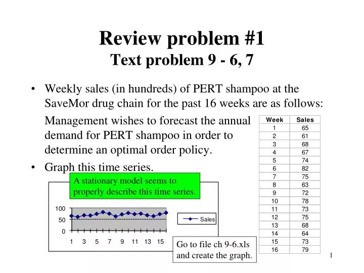
Review problem #1Text problem 9 - 6, 7 • Weekly sales (in hundreds) of PERT shampoo at the SaveMor drug chain for the past 16 weeks are as follows: Management wishes to forecast the annual demand for PERT shampoo in order to determine an optimal order policy. • Graph this time series. A stationary model seems to properly describe this time series. Go to file ch 9-6.xls and create the graph.
Verify statistically that a stationary model is appropriate for forecasting this time series. Do not reject the null hypothesis. There is insufficient evidence for the existence of a trend at (even) 15% significance level. H0: b1= 0 H1: b1¹ 0
Compare the accuracy of the following stationary models: • 3, and 6 period movingaverage • 3 period weighted moving average with optimal weights vs. Exponential smoothing with optimal alpha
Don’t forget to select “Assume non-negative”in “Options” Obtaining the optimal weights 3 - period moving average The sum of the weights appears incell c9.
Don’t forget to select “Assume non-negative”in “Options” The optimal alpha Exponential smoothing model
Review problem #3 A firm that manages and maintains several apartment house complexes has experienced the following expenses over the last five years. Quarter : t 1 2 3 4 5 6 7 8 9 10 11 12 13 14 15 16 17 18 19 20 Yt 27 39 41 50 44 47 58 63 73 92 94 102 123 119 128 147 155 158 164 187 (a) Plot this time series using an Excel graphical tool (use an x-y scatter plot) (b) Run a linear regression model and compare its performance to the best Holt’s model you can obtain, when optimizing alpha and gamma. Use the MAD criterion to compare. (c) Repeat part (b), this time optimize alpha , gamma, the initial forecast and the initial trend. Which model do you select now based on the MAD?
Review problem 3 - Solution • The plot indicates the presence of a linear trend. • Thus, a linear regression model or the Holt’s model should perform well.
The p-value is very small, implying that there is sufficient evidence to support the hypothesis that b1¹0 Review problem 3 - Solution • Running linear regression and checking the p-value of the t-test for b1confirms the observation. The time series has a linear trend.
Review problem 3 – SolutionThe Linear regression Forecasting model
Alpha and gamma are both £ 1 Don’t forget to select “Assume non-negative”in “Options”, since alpha and gamma are both ³ 0 Notice: Only alpha and gamma are optimized Review problem 3 – SolutionOptimizing alpha and gamma For Holt’s
Don’t select “Assume non -negative” in “Options”, since L0 and T0 might be negative. But then, add the non-negativity constraints of alpha and gamma Notice: Both alpha, gamma,L0 and T0 are optimized Review problem 3 - SolutionOptimizing alpha, gamma, L0,T0 for Holt’s
Review problem 3 – Solution • The Holt’s model with all the parameters optimized had the best performance over the past 20 periods based on MAD. • Holt’s (all parameters optimized) MAD = 5.39. • Holt’s (only a and g are optimized) MAD = 6.89 • Linear regression MAD = 7.17
Review problem 4 • Sport King is a chain of 12 sporting goods shops in South Carolina. Total chain demand for the Whamco flying disk averages 250 units a week. While the disks come in various colors, the firm’s policy is to determine the appropriate total order quantity using the EOQ formula and divide this total among the various colors in proportion to historic demand. • Sports King buys the Whamco flying disks for $2.50 each, and sell them for $3.50 each. Sport King uses an annual inventory holding cost rate of 28%, and the cost to place an order is $40. Lead-time for delivery is two weeks, and Sport King desires a safety stock of 50 units.
Problem 4 - continued • Determine: • The optimal order quantity of disks. • The number of calendar days between orders (cycle time). • The reorder point for the disks. • The total annual inventory cost (holding, ordering, procurement) of this policy. • Solution • Annual demand = 250*52 = 13000 disks • Unit holding cost = .28(2.5) = $.7 per unit per year • The optimal order quantity
Problem 4 - continued • The cycle time T = Q*/D • T = Q*/D = 1218.89/13000 = .09376 years = (.09376)(52) = 4.875 weeks = 4.875*7 = 34.129 calendar days. • The reorder point R + Outstanding orders = Lead time demand + safety stock. • R= L*D + SS – Out standing orders • There are no outstanding orders in our problem so:R = 2*(250) + 50 Reorder point 2 weeks 4.875 weeks
Problem 4 - continued • Total annual inventory costs = Procurement cost Ann. Ordering cost Ann. Holding cost
Whamco offers its customers the following all-units price discount schedule:Order Price Value ($) per Unit • 1 – 499$ 2.50 • 500 – 999 $2.25 • 1000–1999 $2.10 • 2000–4999 $1.90 • 5000–9999 $1,80 • $10000 and above $1.75 Quantity Range 1 – ~199 200 - ~399 400 - ~799 800 - ~1999 2000 - ~3999 4000 and above 499/2.5 = 199.6 999/2.5 = 399.6 1999/2.5 = 799.6 Create the order quantity ranges first. Note: All the quantity ranges are calculated based on the original $2.5 per unit. Click to continue.
Assuming that holding costs are discounted, determine the following: • a. The optimal order quantity of Whamco disks. • b. The reorder point for the disks. • c. The number of calendar days between orders (cycle time). • d. The total annual inventory cost (holding, ordering, procurement) for this policy.
Review Problem 5 • The Compland Computer Store sells the HewPacX laser jet printer. Demand has been averaging 24 units per six-day week. The printers cost Compland $1095 each, and Compland uses a 20% annual inventory holding cost rate. The cost of placing an order with HewPac is $90, and the lead time is eight working days. • If Compland runs out of the HewPacX printer, it gives its customers a loaner printer until the next shipment of HewPacX printers arrive. Each loaner costs Compland $1.50 per calendar day. • Determine: • The optimal order quantity of HewPacX printers. • The reorder point for these printers. • The proportion of customers who will get loaner printers. • The total annual inventory cost (holding, ordering, shortage, and procure-ment) of this policy.
Solution D = 24*52 = 1248 per year. Ch = IC = .20(1095) = 219 per unit per year. Co = 90. Cs = 1.50(365) = 547.5 per unit per year. Cb = 0 (not included) • The optimal order quantity = • The reorder point R = LD-S*. The optimal backorder is Then R = 8(24/6) – 10.82 = 21.18
Proportion of customers on backorder (assuming each customer orders one unit) = S*/Q* = 28.6% • Total inventory costs = 27.07 27.89 R = 21 Q = 37.89 8 days Lead time Cycle -10.82 -10.82
Review Problem 6 • Return to the Sports King disk sale problem. • Management has decided to consider uncertainty in the demand pattern. A statistical analysis revealed that the weekly demand is normally distributed with: • mean = 250 disks per week • Standard deviation = 80 disks per week. • Lead time is 2 weeks • Required cycle service level is 92%. • Find • The order quantity, the reorder point, the safety stock • The total inventory costs
2 weeks variance per week • Solution • The order quantity does not change because we assume an EOQ model, as before. • The reorder point depends on the service level. P(DL > R) = .08 P(Z > Z.08) = .08 but Z.08 = 1.405 so (R – m)/s = 1.405 or R = mL + Z.08sL. • Before making the calculation, we need to adjust the mean and standard deviation of the demand during the lead time. mL = 2(250) = 500; sL2 = (2)(80)2 = 12800 sL = 113.13 • Calculating the reorder point: R = 500 + 1.405(113.13) = 658.94 • The safety stock = R – mL = 1.45(113.13) = 164.03 disks.