Download
1 / 35
350 likes | 441 Views
Image Motion. The Information from Image Motion. 3D motion between observer and scene + structure of the scene Wallach O’Connell (1953): Kinetic depth effect

E N D
The Information from Image Motion • 3D motion between observer and scene + structure of the scene • Wallach O’Connell (1953): Kinetic depth effect • Motion parallax: two static points close by in the image with different image motion; the larger translational motion corresponds to the point closer by (smaller depth)
Examples of Motion Fields I (a) (b) (a) Motion field of a pilot looking straight ahead while approaching a fixed point on a landing strip. (b) Pilot is looking to the right in level flight.
Examples of Motion Fields II (a) (b) (c) (d) (a) Translation perpendicular to a surface. (b) Rotation about axis perpendicular to image plane. (c) Translation parallel to a surface at a constant distance. (d) Translation parallel to an obstacle in front of a more distant background.
Assuming that illumination does not change: • Image changes are due to the RELATIVE MOTION between the scene and the camera. • There are 3 possibilities: • Camera still, moving scene • Moving camera, still scene • Moving camera, moving scene
Motion Analysis Problems • Correspondence Problem • Track corresponding elements across frames • Reconstruction Problem • Given a number of corresponding elements, and camera parameters, what can we say about the 3D motion and structure of the observed scene? • Segmentation Problem • What are the regions of the image plane which correspond to different moving objects?
Motion Field (MF) • The MF assigns a velocity vector to each pixel in the image. • These velocities are INDUCED by the RELATIVE MOTION btw the camera and the 3D scene • The MF can be thought as the projectionof the 3D velocities on the image plane.
Motion Field and Optical Flow Field • Motion field: projection of 3D motion vectors on image plane • Optical flow field: apparent motion of brightness patterns • We equate motion field with optical flow field
2 Cases Where this Assumption Clearly is not Valid (a) A smooth sphere is rotating under constant illumination. Thus the optical flow field is zero, but the motion field is not. (b) A fixed sphere is illuminated by a moving source—the shading of the image changes. Thus the motion field is zero, but the optical flow field is not. (a) (b)
Aperture Problem (a) Line feature observed through a small aperture at time t. (b) At time t+t the feature has moved to a new position. It is not possible to determine exactly where each point has moved. From local image measurements only the flow component perpendicular to the line feature can be computed. Normal flow: Component of flow perpendicular to line feature. (a) (b)
Brightness Constancy Equation • Let P be a moving point in 3D: • At time t, P has coords (X(t),Y(t),Z(t)) • Let p=(x(t),y(t)) be the coords. of its image at time t. • Let E(x(t),y(t),t) be the brightness at p at time t. • Brightness Constancy Assumption: • As P moves over time, E(x(t),y(t),t) remains constant.
Brightness Constancy Equation Taking derivative wrt time:
Brightness Constancy Equation Let (Frame spatial gradient) (optical flow) (derivative across frames) and
Brightness Constancy Equation Becomes: vy r E -Et/|r E| vx The OF is CONSTRAINED to be on a line !
Interpretation Values of (u, v) satisfying the constraint equation lie on a straight line in velocity space. A local measurement only provides this constraint line (aperture problem).
Solving the aperture problem • How to get more equations for a pixel? • Basic idea: impose additional constraints • most common is to assume that the flow field is smooth locally • one method: pretend the pixel’s neighbors have the same (u,v) • If we use a 5x5 window, that gives us 25 equations per pixel!
Solution: solve least squares problem • minimum least squares solution given by solution (in d) of: • The summations are over all pixels in the K x K window Constant flow • Prob: we have more equations than unknowns
Taking a closer look at (ATA) The matrix for corner detection: is singular (not invertible) when det(ATA) = 0 But det(ATA) = Õli = 0 -> one or both e.v. are 0 Aperture Problem ! One e.v. = 0 -> no corner, just an edge Two e.v. = 0 -> no corner, homogeneous region
Edge • large gradients, all the same • large l1, small l2
Low texture region • gradients have small magnitude • small l1, small l2
High textured region • gradients are different, large magnitudes • large l1, large l2
Revisiting the small motion assumption • Is this motion small enough? • Probably not—it’s much larger than one pixel (2nd order terms dominate) • How might we solve this problem?
Iterative Refinement • Iterative Lukas-Kanade Algorithm • Estimate velocity at each pixel by solving Lucas-Kanade equations • Warp H towards I using the estimated flow field • - use image warping techniques • Repeat until convergence
u=1.25 pixels u=2.5 pixels u=5 pixels u=10 pixels image H image H image I image I Gaussian pyramid of image H Gaussian pyramid of image I Coarse-to-fine optical flow estimation
warp & upsample run iterative L-K . . . image J image H image I image I Gaussian pyramid of image H Gaussian pyramid of image I Coarse-to-fine optical flow estimation run iterative L-K
Additional Constraints • Additional constraints are necessary to estimate optical flow, for example, constraints on size of derivatives, or parametric models of the velocity field. • Horn and Schunck (1981): global smoothness term • This approach is called regularization. • Solve by means of calculus of variation.
Geometric interpretation Discrete implementation leads to iterative equations
Sources: • Horn (1986) • J. L. Barron, D. J. Fleet, S. S. Beauchemin (1994). Systems and Experiment. Performance of Optical Flow Techniques. IJCV 12(1):43–77. Available at http://www.cs.queesu.ca/home/fleet/ research/Projects/flowCompare.html • http://www.cfar.umd.edu/~fer/postscript/ouchipapernew.ps.gz (paper on Ouchi illusion) • http://www.cfar.umd.edu./ftp/TRs/CVL-Reports-1999/TR4080-fermueller.ps.gz (paper on statistical bias) • http://www.cis.upenn.edu/~beau/home.html http://www.isi.uu.nl/people/michael/of.html (code for optical flow estimation techniques)