Download
1 / 16
180 likes | 326 Views
Eng. 6002 Ship Structures 1 Hull Girder Response Analysis. Introduction to Maple. Overview. PURPOSE: To illustrate the use of dsolve to find exact solutions of many differential equations or systems of equations, with or without initial conditions.

E N D
Eng. 6002 Ship Structures 1Hull Girder Response Analysis Introduction to Maple
Overview • PURPOSE: To illustrate the use of dsolve to find exact solutions of many differential equations or systems of equations, with or without initial conditions. • NOTE 1. Maple has a powerful symbolic differential equation solver called dsolve. This command directs Maple to seek an exact symbolic expression for the solution of a given differential equation, or a system of differential equations, with or without initial conditions. • NOTE 2. Further information about dsolve can be obtained by issuing the command ‘?dsolve’.
Overview cont. • IMPORTANT NOTE: dsolve insists that coefficients be entered as rational, rather than floating point, numbers. For example, you should enter a coefficient as 1/2 or 1/4, rather than 0.5 or 0.2.
Example 1: A 1st order linear equation • Find the general solution of the differential equation dy/dt = -2 + sin(t) - (1/4)y. • Also find the solution that satisfies the initial condition y(0) = 2. • SOLUTION. The first step is to enter the differential equation. • eq1 := diff(y(t),t) = -2 + sin(t) - 1/4*y(t);
Example 1: A 1st order linear equation • Now dsolve can be used to find the general solution of this equation. • In its simplest form the command has two arguments; • the first is the equation to be solved • the second is the variable to be solved for. • dsolve(eq1,y(t));
Example 1: A 1st order linear equation • This is the general solution of the given differential equation. Note that Maple writes the arbitrary constant as _C1, and that in this case the constant follows the term exp(-t/4) that it multiplies. • To find the solution that also satisfies the initial condition, we include the initial condition in the dsolve command, using braces to delimit the problem to be solved. Also we assign the name sol to the result. • sol := dsolve({eq1,y(0)=2},y(t));
Example 1: A 1st order linear equation • We can now assign a name, if we wish, to the expression for y(t) on the right side of the last result, as follows: • > y1 := rhs(sol); • This enables us to perform operations on the solution y1 of the initial value problem. For instance, we can evaluate y1 at a given value of t, or we can plot y1 on some given t interval. • > evalf(subs(t=4,y1));
Example 1: A 1st order linear equation • plot(y1,t=0..20);
Example 2: A 2nd order homogeneous linear equation • Solve the equation y’’ - 2y’ - 4y = 0. • Find the general solution and also the solution that satisfies the initial conditions y(0) = 2, y’(0) = -7/4. • SOLUTION: Again the first step is to enter the differential equation. In the following command note that the first term the second derivative is entered using t$2. This causes the differentiation operation to be executed twice. • eq2 := diff(y(t),t$2) - 2*diff(y(t),t) - 4*y(t) = 0; • dsolve(eq2,y(t));
Example 2: A 2nd order linear equation • This is the general solution. Note that it contains two exponential terms, each multiplied by an arbitrary constant. One of the exponentials is positive, and so grows with increasing t, while the other is negative, and decays as t increases. • Now we solve the initial value problem. To enter the second initial condition, denote y’(0) by D(y)(0). We will assign the name y2 to this solution, combining the dsolve and rhs commands. • > y2 := rhs(dsolve({eq2,y(0) = 2,D(y)(0)=-7/4},y(t)));
Example 3: A 2nd order non-homogeneous linear equation • Find the general solution of the equation y’’ + 4 y’ + 5 y = 3 exp(-t) + 4 sin(3t). • Also find the solution satisfying the initial conditions • y(0) = 3/2, y’(0) = 2, and plot its graph. • SOLUTION. As in the preceding examples we find the general solution by entering the equation and then using dsolve. • > eq3 :=diff(y(t),t$2)+4*diff(y(t),t)+5*y(t)=3*exp(-t)+4*sin(3*t);
Example 3: A 2nd order non-homogeneous linear equation • sol := dsolve(eq3,y(t)); • init := y(0) = 3/2, D(y)(0) = 2; • sol := dsolve({eq3,init},y(t)): • plot(y3,t=0..15);
Example 4: Find the general solution of a system • Find the general solution of the system dx/dt = -2 x + y, dy/dt = x - 2 y. • Also find the solution that satisfies the initial conditions x(0) = 0, y(0) = 2. • sys := diff(x(t),t) = -2*x(t)+y(t), diff(y(t),t) = x(t) - 2*y(t); • dsolve({sys},{x(t),y(t)});
Example 4: Find the general solution of a system • Here is the solution of the initial value problem. • > dsolve({sys,x(0)=0,y(0)=2},{x(t),y(t)});
Ass 2 • In each of the following problems use dsolve to find the general solution of the given differential equation. If initial conditions are given, also find the solution that satisfies them. • Plot this solution.
Ass 2 cont. • 1. dy/dt = t + exp(-2t) + 3y, y(0) = 2 • 2. dy/dt = 3 sin(t) + 1 - y, y(0) = -1 • 3. y’’ + (5/2)y’ + y = 0, y(0) = 2, y’(0) = 3 • 4. y’’ + 6y’ + 10y = 0, y(0) = 1, y’(0) = 1 • 5. y’’ + (5/2)y’ + y = 3 cos(2t) + 6 exp(-2t), y(0) = 2, y’(0) = 3 • 6. y’’ + 6y’ + 10y= 5 exp(-3t)cos(t) + 2 exp(-t)cos(3t), y(0) = 1, y’(0) = 2 • 7. y’’’ + 3y’’ + 3y’ + 2y = 0,y(0) = 2, y’(0) = -1, y’’(0) = 3 • 8. y’’’’ + 4y’’’ + 10y’’ + 11y’ + 10y = 0, y(0) = 2, y’(0) = 3, y’’(0) = -1, y’’’(0) = 0 • 9. y’’’ + 3y’’ + 3y’ + 2y = exp(-t)sin(t) + 3t^2 - 4t + 5, y(0) = 2, y’(0) = -1, y’’(0) = 3 • 10. dx/dt = 3x - 2y, dy/dt = 2x - 2y,x(0) = 3, y(0) = 2