Download
1 / 90
920 likes | 1.1k Views
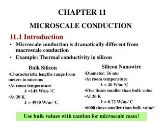
11.1 Introduction. CHAPTER 11. MICROSCALE CONDUCTION. Microscale conduction is dramatically different from macroscale conduction Example: Thermal conductivity in silicon. Silicon Nanowire Diameter: 56 nm At room temperature k = 26 W/m-°C Five times smaller than bulk value

E N D
11.1 Introduction CHAPTER 11 MICROSCALE CONDUCTION • Microscale conduction is dramatically different from macroscale conduction • Example: Thermal conductivity in silicon • Silicon Nanowire • Diameter: 56 nm • At room temperaturek = 26 W/m-°C • Five times smaller than bulk value • At 20 Kk = 0.72 W/m-°C • 6000 times smaller than bulk value! • Bulk Silicon • Characteristic lengths range from meters to microns • At room temperaturek =148 W/m-°C • At 20 Kk = 4940 W/m-°C Use bulk values with caution for microscale cases!
11.1.1 Categories of Microscale Phenomena • Classical Fourier law of diffusive heat conduction breaks down for • processes that are too fast • systems that are too small • Chapter focus is on small systems at steady-state • Essential questions • What are the physical mechanisms by which the classical Fourier’s law will fail for small systems? • At what length scales does this happen? • How can we modify Fourier’s law to still be useful at the microscale? • What is the effective thermal conductivity k for a microstructure such as a nanowire or thin film?
Fig. 11.1 • Wavepacket (Fig. 11.1.a) • A wavelike disturbance localized within a small volume of space • Particle-like “Wavepacket” concept and classical size effect l = wavepacket wavelength L = mean free path L = characteristic length • When l << L << L, wavepacket is treated as a particle (Fig. 11.1.b) • Classical size effect (Fig. 11.1.c) • When L > L >> l, boundary collisions increase, impeding energy flow • Particle approximation still holds
11.1.2 Purpose and Scope of this Chapter • Steady-state heat conduction at the microscale • Key concepts of the classical size effect • Supporting subjects not covered • Solid state physics • Quantum mechanics • Statistical thermodynamics 11.2 Understanding the Essential Physics of Thermal Conductivity Using the Kinetic Theory of Gases • Kinetic theory offers • Maximum physical insight for minimal complexity • Applicable to a wide range of realistic problems
Fig. 11.2.a through 11.2.c (11.1) 11.2.1 Derivation of Fourier’s Law and an Expression for the Thermal Conductivity • Energy is exchanged when particles collide • “Mean free path” is the average of the distances a particle travels between collisions • L = mean free path • “Mean free time” is the corresponding time between collisions • t = mean free time
Fig. 11.2.d Derivation of Fourier’s Law by net energy flow evaluation • Consider two adjacent control volumes of gas each with thickness L and area A, subject to a temperature gradient, Fig. 11.2.d • After waiting a period t = L/v, half the particles in each control volume have exited through the boundaries • Particles from the left are hotter than particles from the right ESTIMATION OF ENERGY EXCHANGE Total energy in the left control volume:
Total energy in the right control volume: Note that Uavg is the internal energy per unit volume, J/m3 The net energy crossing x = x0 is Assuming U is a smoothly-varying function of x that is approximated as a straight line over distance L:
(11.2) Using a Taylor series expansion: • Assumption of local thermodynamic equilibrium: • energy density of the particles conforms to the local temperature Exact analysis shows that the correct expression is: By the chain rule of calculus: where C is the specific heat capacity at constant volume per unit volume
(11.3) (11.4) Collecting results, dividing by the area and elapsed time yields Fourier’s law of heat conduction: Therefore, the thermal conductivity of a gas of particles is: 11.3 Energy Carriers • Section focus: Identify the particles in a heat-conducting material that carry the energy • Determine the following properties: C, v, L • Ideal gas, metal, insulators and heat transfer by radiation will be investigated
Recall the ideal gas law (11.5) (11.6) 11.3.1 Ideal Gases: Heat is Conducted by Gas Molecules where p = absolute pressure V = volume mtot= total mass of the gas T = absolute temperature in Kelvin R = gas constant for the gas being studied, found from: where RU= universal gas constant, 8.314 J/mol-K M = molecular weight of the gas
(11.7) (11.8) • Also recall that the universal gas constant can be expressed as: where NA = Avogadro’s number, 6.022 x 10²³ mol-1 kB = Boltzmann’s constant, 1.381 x 10⁻²³ J/K Use absolute temperature units throughout this chapter Properties of monoatomic gases • Specific heat • Specific heats at constant volume (cV) and constant pressure (cp) are related by: • On a per-unit-volume basis they are related by:
(11.9) (11.10) • The specific heat has the form: • Speed • Molecular speeds are distributed over a broad range of values: the Maxwellian velocity distribution • This distribution is temperature dependent • Thermal velocity is represented by the root-mean-square velocity: • Mean Free Path • Mean free path between collisions is:
(11.11) where is the average number of molecules per unit volume d = effective diameter of the gas molecule • Not all energy is exchanged during molecule collisions • The mean free path for energy exchange is: Note that Len is about 3.5 times larger than Lcoll, and Len is the correct choice for evaluating thermal conductivity.
(1) Observations (2) Formulation Example 11.1: Thermal Conductivity of an Ideal Gas Calculate the thermal conductivity for helium at 0°C and atmospheric pressure and compare with experimental value from Appendix D. Molecular diameter of He:d = 0.2193 nm • Helium is a monoatomic gas • Kinetic gas theory applies • Assumptions • (1) Helium can be modeled as an ideal monoatomic gas • (2) atoms are treated as elastic spheres
(b) (a) (c) (d) • Governing Equations • Kinetic theory expression, (11.4) Expression for C, (11.9) Expression for v, (11.10) Expression for L, (11.11)
(3) Solution • Specific heat: • Substituting T = 273.15 K and p = 101,300 pa into (b) yields: Note that 1 Pa = 1 J/m3 • Speed: • Atomic weight of He: M = 4.003 g/mol, so • Substituting R and T into (c) yields:
Mean free path: • Substituting numeric values into (d) yields: • Thermal conductivity: • Substituting the values for Cv, v and L into (a) yields:
(4) (5) Checking Comments • Comparison with experimental value: • Experimental value for thermal conductivity for He at 0°C from Appendix D: 0.142 W/m-°C • Dimensional Check • Units of CvL are (J-m-3-°C-1)(m-s-1)(m), which gives (W/m-°C) – the correct units for k • Observed 3.1% error in k is only slightly larger than the 2% uncertainty stated in (11.11) for L and reflects the experimental uncertainty in d and k
Since helium’s diameter is smaller than that of all other gases, the value of L is a relatively large value for an ideal gas • Molecules with larger diameters have smaller L • Helium gas used to conduct heat between two parallel plates with a gap less than the mean free path will be discussed later in the chapter • This refers to “classical size effect” 11.3.2 Metals: Heat is Conducted by Electrons • Metals have high concentrations of “free electrons” that are • Responsible for high thermal conductivity • Dominate transporters of heat • Theoretical results are presented
(11.12) Properties of electrons in metals • Speed • Electrons travel at the same speed, known as the Fermi velocity vF • Typical values of vF are around 1-2 x 10⁶ m/s • Free electrons are also characterized by their Fermi Energy EF, related to vF by where me is the mass of an electron: 9.110 x 10⁻³¹ kg • Fermi velocity is related to the concentration of free electrons he by where is the reduced Planck’s constant
(11.13) (11.14) • Specific heat • Simple form, expressed in three ways: • Second form of (11.13) defines a characteristic “Fermi Temperature” • Third form of (11.13) shows specific heat is proportional to temperature • Coefficient g has units of J/m3-K2 • Though electrons dominate thermal conductivity, Ce is typically several orders of magnitude smaller than reference values of C for metals
Mean free path • Typically on the order of tens of nm at room temperature • Free electron properties of selected metals (Table 11.1)
(11.15) 11.3.3 Electrical Insulators and Semiconductors: Heat is Conducted by Phonons (Sound Waves) • Insulators (dielectrics) have extreme scarcity of electrons as compared to metals • Atomic vibrations store thermal energy • Sound waves are the simplest class of atomic vibrations • Wavelengths of sound waves are much larger than lattice spacing between atoms • Wavelength l and oscillation frequency w follow the simple relationship where vs is the speed of sound in the material A “phonon” is the quantum of a sound wave in the same way that a “photon” is the quantum of a light wave
There are two classes of phonons: acoustic and optical • Acoustic phonons are sound waves that follow (11.15) with an upper limit on the allowed frequencies • At sufficiently high frequencies, the wavelengths become comparable to the lattice constant, and it is unphysical to speak of wavelengths shorter than twice the interatomic spacing • Optical phonons are present if and only if a material’s crystal structure has more than one atom per “primitive unit cell” • The velocity of optical phonons is commonly set to zero, implying that optical phonons make negligible contribution to heat transfer • Acoustic phonons will be the exclusive focus with regard to thermal conductivity
(11.16) Properties of Acoustic Phonons • The approximations used here are the Debye approximations • Speed • Acoustic phonons are approximated by traveling at the speed of sound, vs, in the material • This is found by averaging the transverse and longitudinal sound speeds: • The above ensures that the result becomes exact at low temperature
(11.17) (11.18) • Specific heat • Approximation to exact Debye calculation: where hPUC is the number of primitive cell units and qD is the “Debye temperature:” • Equation (11.17) gives less than 12% error compared to the exact Debye calculation at intermediate temperatures • A slightly different definition of qD substitutes hPUC with the number density of atoms hatoms
(11.19) (11.20) • In the limits of high and low temperature, eq. (11.17) reduces to the well-known limiting expressions • In equation (11.19), low temperature result, C is proportional to T3 : the “Debye T3 law” • In equation (11.20), high temperature result, C approaches a constant: the “Law of Dulong and Petit” • An “Einstein model” is used for specific heat for optical phonons • Handbook values for C are for total specific heat which includes contributions from both acoustic and optical phonons
Mean free path • Like electrons, phonon mean free path in many insulators is approximately proportional to T-1 • At room temperature and above, thermal resistance is dominated by phonons scattering with other phonons • Alloy atoms can also result in strong phonon scattering • Example: Ge atoms in a crystal with composition Si0.9Ge0.1 • Dopant atoms in a “doped” crystal can scatter phonons • At temperatures around 300 K and below, effects of phonon scattering off of impurities, isotopes, defects and grain boundaries may also need to be considered • Phonons can also scatter off sample boundaries • Classical size effect • Discussed later in the chapter
(1) Observations Example 11.2: Thermal Conductivity Trend with Temperature for Silicon Use data from Table 11.2 to propose a power law approximation of the form k(T) = aT b, where a and b are constants for thermal conductivity of bulk silicon Assume mean free path proportional to T-1 Temperature range is 300K to 1000K • Thermal conductivity of silicon has been well-studied over a broad range of temperatures • Example limits us to the information in Table 11.2
(2) (3) Formulation Solution • Assumptions • (1) Thermal conductivity is dominated by acoustic phonons, so Debye model is adequate • (2) Specific heat can be approximated by the high-T limit since the temperatures of interest are greater than qD/2 • (3) The mean free path is assumed to vary inversely proportional to temperature • Governing Equations • Specific heat of acoustic phonons, eq. (11.20) Speed: From Table 11.2:
Specific heat: • Using values from Table 11.2 in (11.20) yields: • C is assumed constant from 300 K to 1000 K • Thermal conductivity at 300 K: • From Table 11.2: • Mean free path: • Combining values for k, C and v at 300K:
Since L varies in proportion to T -1: • Thermal conductivity power law: • Consider k(T)/k(300K) • From kinetic theory: • Since C is approximately constant:
Using the result for L: • The final result is: • Comparing to the power law form: • where T must be expressed in Kelvin
(4) (5) Checking Comments • Dimensional Check • Right hand side of last eq. has units of K-1-W/m which is equivalent to expected units of W/m-°C • Magnitude Check • Calculations are compared to standard reference values from Appendix D: • Mean free path is best measured in nm; values in the range of tens to hundreds of nm are typical for phonons in dielectric crystals at room temperature
Using density of silicon r = 2330 kg/m3 from Appendix D, acoustic specific heat is converted to a mass basis, yielding 446 J/kg-°C • Handbook value in Appendix D is 712 J/kg-°C • Optical phonons make a significant contribution to the total specific heat • The T-1 power law is only approximate • Actual thermal conductivity varies by a factor of 4.74, compared to the expected variation by a factor of 3.33 • A better power law in this range is • (iv) Power law is strongly temperature dependent • Below 10 K, power law is
(1) Observations Example 11.3: Bulk Mean Free Paths as a Function of Temperature Estimate L for acoustic phonons in bulk silicon as a function of temperature Temperature range is 1 K to 1000 K Use approximate Debye model for specific heat and sound velocity Thermal conductivity of bulk silicon from Appendix D • Temperature range is both far above and far below qD • Above room temperature, phonon-phonon scattering dominates the mean free path with an approximate power law of
(2) Formulation • At low temperature, thermal conductivity climbs as T is reduced from 300 K to 20 K, but then falls rapidly as T is further reduced • Assumptions • (1) Thermal conductivity is dominated by acoustic phonons over the entire range • (2) The Debye model is adequate • Governing Equations • Specific heat eq. (11.17) will be used Sound velocity is taken from Table 11.2
(3) Solution Mean free path is given by From equation (11.17) where from Table 2: Mean free path is calculated by combining the above with the data for k from Appendix D.
Fig. 11.3 Tabulated and graphical results:
(4) Checking • Limiting Behavior Check • The specific heat transitions from T 3 at low temperature to constant at high temperature, as expected • Transition occurs at 120 K, which is near the expected transition of qD/3 = 170 K • Trends of both mean free path and thermal conductivity are approximately T -1 at high temperature, as expected • Value Check • At 300 K, C is 9.73 x 10⁵ J/m3-°C, which is close to 1.04 x 10⁶ J/m-°C found in Ex. 11.2 using high-temperature approximation • L is 78 nm, which is close to 73 nm found in Ex. 11.2
(5) Comments • Low-temperature behavior is distinctive • Mean free path appears to saturate at 4 nm • Since low-temperature specific heat goes as T 3, so does the low-temperature thermal conductivity • Cubic trend is general for phonon thermal conductivity at low temperature • Behavior is dominated by classical size effect at low temperature • L of 4 nm corresponds to characteristic length of sample used to generate values of k in Appendix D • Other reference values for bulk silicon at low temperatures may differ due to sample size, but high temperature values should correlate well
(11.21) 11.3.4 Radiation: Heat is Carried by Photons (Light Waves) • Using kinetic theory, radiation and conduction are seen as two limiting cases of a single phenomenon • Radiation is treated as a gas of photons • Speed • Speed of light in vacuum is c = 2.998 x 10⁸ m/s • Specific heat • Photons store energy similarly to molecules, electrons and phonons • Assuming perfect vacuum conditions, specific heat of a “gas” of photons is where s is the Stephan-Boltzmann constant, 5.670 x 10⁻⁸ W/m2-K4
Mean free path • Varies tremendously • Much longer than that of molecules, electrons and phonons • Depends on physical situation • Sun surface to earth: 90 million miles without scattering • Vacuum chamber: mean free path is on order of 10-100 mm • Crystals transparent in infrared (i.e. glasses): mean free path is dependent on wavelength and material, magnitude is microns to mm
(11.22) Example 11.4: Effective Thermal Conductivity for Radiation Heat Transfer Between Two Parallel Plates (One Black, One Gray) Net radiation heat transfer from a gray plate “1” to a parallel black plate “2” is: where e is the emissivity of plate 1 the plates have the same area A the gap L is smaller than the length and width Use kinetic theory to re-express heat transfer in terms of a “conduction thermal resistance” R = L/kradA where krad is the effective thermal conductivity of a photon gas Derive effective mean free path Assume temp. differences are smaller than average temp. Evaluate for A = 0.1m2, L = 0.001m, e = 0.2, T1 = 600 K, T2 = 500 K
(1) Observations (2) Formulation • Since there is an expression for the speed and specific heat of photons, it should be possible to express radiation as conduction • In a vacuum, there are no scattering mechanisms other than the plates themselves, so the photon mean free path should be proportional to L • Assumptions • (1) Small temperature differences: (2) Properties such as specific heat can be evaluated at the average temperature:
(3) Solution • Governing Equations • Radiation heat transfer equation (11.22): Kinetic theory equation (11.4): Specific heat of photons (11.21): Conduction resistance Equation (11.22) is to be rearranged into the form: where R is the desired conduction resistance
Define the temperature difference: Therefore: Substituting the above into (11.22): Factoring out T 4: From the binomial theorem or Taylor series expansion: So, since D << T:
(11.23) Then Simplifying: which is rearranged: The conduction resistance is therefore: Effective thermal conductivity Comparing (11.23) to the standard form R = L/kA, solve for k:
(11.24) Effective mean free path Comparing krad to the standard form (11.4), solve for Leff : Substituting (11.21) for C, and recognizing v = c: Numerical calculation From the exact radiation equation, Q = 76.1 W From conduction resistance equation with T = 550K, R = 1.33 K/W, resulting in Q = 75.5 W This is within 1% of the exact value