Download
1 / 66
660 likes | 783 Views
Feedback: The simple and best solution. Applications to self-optimizing control and stabilization of new operating regimes. Sigurd Skogestad Department of Chemical Engineering Norwegian University of Science and Technology (NTNU) Trondheim. Austin Nov. 2006. Abstract.

E N D
Feedback:The simple and best solution.Applications to self-optimizing control and stabilization of new operating regimes Sigurd Skogestad Department of Chemical Engineering Norwegian University of Science and Technology (NTNU) Trondheim Austin Nov. 2006
Abstract • Feedback: The simple and best solution • Applications to self-optimizing control and stabilization of new operating regimes • Sigurd Skogestad, NTNU, Trondheim, Norway • Most chemical engineers are (indirectly) trained to be “feedforward thinkers" and they immediately think of “model inversion'' when it comes doing control. Thus, they prefer to rely on models instead of data, although simple feedback solutions in many cases are much simpler and certainly more robust.The seminar starts with a simple comparison of feedback and feedforward control and their sensitivity to uncertainty. Then two nice applications of feedback are considered: 1. Implementation of optimal operation by "self-optimizing control". The idea is to turn optimization into a setpoint control problem, and the trick is to find the right variable to control. Applications include process control, pizza baking, marathon running, biology and the central bank of a country. 2. Stabilization of desired operating regimes. Here feedback control can lead to completely new and simple solutions. One example would be stabilization of laminar flow at conditions where we normally have turbulent flow. I the seminar a nice application to anti-slug control in multiphase pipeline flow is discussed.
Outline • About Trondheim • I. Why feedback (and not feedforward) ? • II. Self-optimizing feedback control: What should we control? • III. Stabilizing feedback control: Anti-slug control • Conclusion • More information:
Arctic circle North Sea Trondheim SWEDEN NORWAY Oslo DENMARK GERMANY UK
NTNU, Trondheim
Outline • About Trondheim • I. Why feedback (and not feedforward) ? • II. Self-optimizing feedback control: What should we control? • III. Stabilizing feedback control: Anti-slug control • Conclusion
k=10 time 25 Example 1 d Gd G u y Plant (uncontrolled system)
d Gd G u y
Model-based control =Feedforward (FF) control d Gd G u y ”Perfect” feedforward control: u = - G-1 Gd d Our case: G=Gd → Use u = -d
d Gd G u y Feedforward control: Nominal (perfect model)
d Gd G u y Feedforward: sensitive to gain error
d Gd G u y Feedforward: sensitive to time constant error
d Gd G u y Feedforward: Moderate sensitive to delay (in G or Gd)
d Gd ys e C G u y Measurement-based correction =Feedback (FB) control
d Gd ys e C G u y Output y Input u Feedback generates inverse! Resulting output Feedback PI-control: Nominal case
d Gd ys e C G u y Feedback PI control: insensitive to gain error
d Gd ys e C G u y Feedback: insenstive to time constant error
d Gd ys e C G u y Feedback control: sensitive to time delay
Comment • Time delay error in disturbance model (Gd): No effect (!) with feedback (except time shift) • Feedforward: Similar effect as time delay error in G
Conclusion: Why feedback?(and not feedforward control) • Simple: High gain feedback! • Counteract unmeasured disturbances • Reduce effect of changes / uncertainty (robustness) • Change system dynamics (including stabilization) • Linearize the behavior • No explicit model required • MAIN PROBLEM • Potential instability (may occur “suddenly”) with time delay/RHP-zero
Outline • About Trondheim • Why feedback (and not feedforward) ? • II. Self-optimizing feedback control: What should we control? • Stabilizing feedback control: Anti-slug control • Conclusion
Optimal operation (economics) • Define scalar cost function J(u0,d) • u0: degrees of freedom • d: disturbances • Optimal operation for given d: minu0 J(u0,x,d) subject to: f(u0,x,d) = 0 g(u0,x,d) < 0
”Obvious” solution: Optimizing control =”Feedforward” Estimate d and compute new uopt(d) Probem: Complicated and sensitive to uncertainty
Engineering systems • Most (all?) large-scale engineering systems are controlled using hierarchies of quite simple single-loop controllers • Commercial aircraft • Large-scale chemical plant (refinery) • 1000’s of loops • Simple components: on-off + P-control + PI-control + nonlinear fixes + some feedforward Same in biological systems
In Practice: Feedback implementation Issue: What should we control?
RTO y1 = c ? (economics) MPC PID Further layers: Process control hierarchy
Implementation of optimal operation • Optimal solution is usually at constraints, that is, most of the degrees of freedom are used to satisfy “active constraints”, g(u0,d) = 0 • CONTROL ACTIVE CONSTRAINTS! • Implementation of active constraints is usually simple. • WHAT MORE SHOULD WE CONTROL? • We here concentrate on the remaining unconstrained degrees of freedom.
Optimal operation Cost J Jopt copt Controlled variable c
Optimal operation Cost J d Jopt n copt Controlled variable c Two problems: • 1. Optimum moves because of disturbances d: copt(d) • 2. Implementation error, c = copt + n
Effect of implementation error Good Good BAD
Self-optimizing Control • Define loss: • Self-optimizing Control • Self-optimizing control is when acceptable operation (=acceptable loss) can be achieved using constant set points (cs)for the controlled variables c (without the need for re-optimizing when disturbances occur). c=cs
Self-optimizing Control – Sprinter • Optimal operation of Sprinter (100 m), J=T • Active constraint control: • Maximum speed (”no thinking required”)
Self-optimizing Control – Marathon • Optimal operation of Marathon runner, J=T • Any self-optimizing variable c (to control at constant setpoint)?
Self-optimizing Control – Marathon • Optimal operation of Marathon runner, J=T • Any self-optimizing variable c (to control at constant setpoint)? • c1 = distance to leader of race • c2 = speed • c3 = heart rate • c4 = level of lactate in muscles
Self-optimizing Control – Marathon • Optimal operation of Marathon runner, J=T • Any self-optimizing variable c (to control at constant setpoint)? • c1 = distance to leader of race (Problem: Feasibility for d) • c2 = speed (Problem: Feasibility for d) • c3 = heart rate (Problem: Impl. Error n) • c4 = level of lactate in muscles (Problem: Impl.error n)
Further examples • Central bank. J = welfare. u = interest rate. c=inflation rate (2.5%) • Cake baking. J = nice taste, u = heat input. c = Temperature (200C) • Business, J = profit. c = ”Key performance indicator (KPI), e.g. • Response time to order • Energy consumption pr. kg or unit • Number of employees • Research spending Optimal values obtained by ”benchmarking” • Investment (portofolio management). J = profit. c = Fraction of investment in shares (50%) • Biological systems: • ”Self-optimizing” controlled variables c have been found by natural selection • Need to do ”reverse engineering” : • Find the controlled variables used in nature • From this possibly identify what overall objective J the biological system has been attempting to optimize
Candidate controlled variables c for self-optimizing control Intuitive • The optimal value of c should be insensitive to disturbances (avoid problem 1) • Optimum should be flat (avoid problem 2 – implementation error). Equivalently: Value of c should be sensitive to degrees of freedom u. “Want large gain” Charlie Moore (1980’s): Maximize minimum singular value when selecting temperature locations for distillation
Mathematical: Local analysis cost J c = G u u uopt
Minimum singular value of scaled gain Maximum gain rule (Skogestad and Postlethwaite, 1996): Look for variables that maximize the scaled gain (Gs) (minimum singular value of the appropriately scaled steady-state gain matrix Gsfrom u to c)
Self-optimizing control: Recycle processJ = V (minimize energy) 5 4 1 Given feedrate F0 and column pressure: 2 3 Nm = 5 3 economic (steady-state) DOFs Constraints: Mr < Mrmax, xB > xBmin = 0.98 DOF = degree of freedom
Recycle process: Control active constraints Active constraint Mr = Mrmax Remaining DOF:L Active constraint xB = xBmin One unconstrained DOF left for optimization: What more should we control?
Maximum gain rule: Steady-state gain Conventional: Looks good Luyben snow-ball rule: Not promising economically
Recycle process: Loss with constant setpoint, cs Large loss with c = F (Luyben rule) Negligible loss with c =L/F or c = temperature
Recycle process: Proposed control structurefor case with J = V (minimize energy) Active constraint Mr = Mrmax Active constraint xB = xBmin Self-optimizing loop: Adjust L such that L/F is constant
Outline • About myself • Why feedback (and not feedforward) ? • Self-optimizing feedback control: What should we control? • III. Stabilizing feedback control: Anti-slug control • Conclusion
Application stabilizing feedback control:Anti-slug control Two-phase pipe flow (liquid and vapor) Slug (liquid) buildup
Slug cycle (stable limit cycle) Experiments performed by the Multiphase Laboratory, NTNU