Download
1 / 12
120 likes | 224 Views
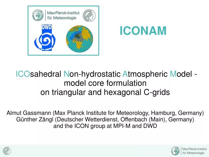
ICONAM. ICO sahedral N on-hydrostatic A tmospheric M odel - model core formulation on triangular and hexagonal C-grids Almut Gassmann (Max Planck Institute for Meteorology, Hamburg, Germany) Günther Zängl (Deutscher Wetterdienst, Offenbach (Main), Germany)

E N D
ICONAM ICOsahedral Non-hydrostatic Atmospheric Model - model core formulation on triangular and hexagonal C-grids Almut Gassmann (Max Planck Institute for Meteorology, Hamburg, Germany) Günther Zängl (Deutscher Wetterdienst, Offenbach (Main), Germany) and the ICON group at MPI-M and DWD
ICON: tool for NWP and climate applications Wishes for the project some years ago: • non-hydrostatic atmospheric model • dynamics in grid point space • triangular icosahedron grid • local zooming with static or dynamic grid refinement • transport scheme: conservative, positive definit, efficient • dynamics conserves mass, energy, potential vorticity, and potential enstrophy • coupling to ocean model, atmospheric chemistry, hydrology, and land model • modulartity • portability • scalability and efficiency on multicore architectures from: http://infoskript.de/uploads/pics/Wollmilchsau.jpg
prognostic equations Non-hydrostatic atmospheric model - model core formulation Target system of equations: |·ρv (to obtain energy equ.) Π = Exner pressure θv = virtual pot. temperature ρ = density v = 3D velocity vector K = spec. kinetic energy Φ = geopotential ωa = 3D abs. vorticity vector Rd = gas constant for dry air cvd = spec. heat capacity at constant volume for dry air cpd = spec. heat capacity at constant pressure for dry air +physics Transport of virtual potential temperature is done with higher order advection. Additional transport equations for tracers will enter the system.
Triangular and hexagonal C-grids • Hexagonal C-grid • no divergence averaging • C-grid dispersion properties retained • 14-point tangential wind reconstruction • 3D vector invariant form • conserves mass and energy • needs diffusion for nonlinear processes • 3rd order upstream advection for θ • static grid refinement not yet implemented • still farther away from operational availability • Triangular C-grid • divergence averaging • C-grid dispersion properties lost • 4-point tangential wind reconstruction • horizontally (2D) vector invariant form • conserves mass • needs diffusion for stability • Miura advection for ρand ρθ • static grid refinement implemented • nearer to operational availability
Triangular and hexagonal C-grids Further distinguishing features of the two model versions: a) implementation of terrain-following coordinates b) time stepping scheme
a) L-grid staggering + terrain-following coordinates • Triangular C-grid • main levels height-centered between interface levels • horizontal pressure gradient: • search for neighboring point in the same height • reconstruct Exner function using a second order Taylor expansion w m w
a) L-grid staggering + terrain-following coordinates • Hexagonal C-grid • interface levels height-centered between main levels • horizontal pressure gradient: • covariant velocity equations • remove background reference profile in each of them separately • solve inverse problem for the lower boundary w m w
a) Acid test for terrain-following coordinates: Resting atmosphere over a high mountain Vertical slice model based on the hexagonal C-grid code Spurious vertical velocities remain in the range of mm/s. No errors spoil higher levels, compared to other models.
b) Time stepping scheme • Common features • horizontally explicit (forward-backward) for waves • vertically implicit scheme for waves • no time splitting • Triangular C-grid • Adams-Bashford-Moulton time stepping for momentum advection • Hexagonal C-grid • approximately conserves energy (integration by parts rule in time) • resembles in parts the Matsuno scheme (needs v(n+1) for the kinetic energy term)
Density current Vertical slice model based on the hexagonal C-grid code Essential feature: Higher order transport for potential temperature. Here: 3rd order upstream
Results for global testcases: Talk by Pilar Ripodas (DWD) Grid refinement (triangular C-grid): Talk by Günther Zängl (DWD) • Next steps • implementation of physics parameterizations which are available from the COSMO model (DWD) • hydrostatic version: implementation of ECHAM physics (MPI-M) • grid refinement also for hexagonal C-grid version • coupling to ocean model (under development at MPI-M) • available for preoperational NWP runs next year