Download
1 / 4
40 likes | 158 Views
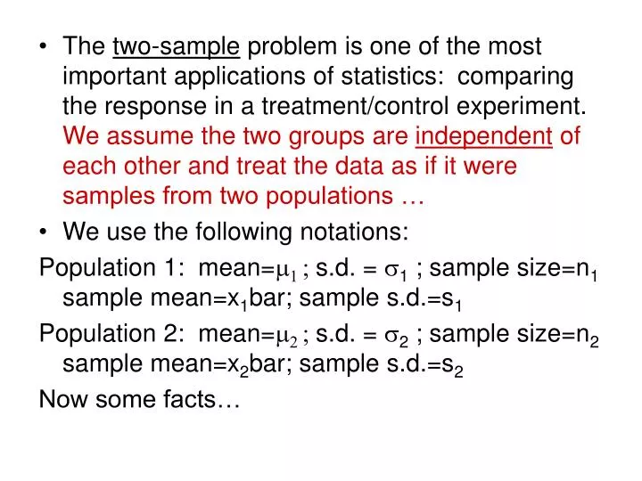
The two-sample problem is one of the most important applications of statistics: comparing the response in a treatment/control experiment. We assume the two groups are independent of each other and treat the data as if it were samples from two populations … We use the following notations:

E N D
The two-sample problem is one of the most important applications of statistics: comparing the response in a treatment/control experiment. We assume the two groups are independent of each other and treat the data as if it were samples from two populations … • We use the following notations: Population 1: mean=m1 ; s.d. = s1 ; sample size=n1 sample mean=x1bar; sample s.d.=s1 Population 2: mean=m2 ; s.d. = s2 ; sample size=n2 sample mean=x2bar; sample s.d.=s2 Now some facts…
x1bar – x2bar is N(m1 - m2 , sqrt(s12/n1 + s22/n2 )) so we may use it as a basis for constructing confidence intervals for m1 - m2 and for testing hypotheses about m1 - m2 . • As you might guess, the population standard deviations are rarely known, so we usually estimate them with s12 and s22 … the resulting statistic is called the two-sample t statistic and is given at the bottom of page 488 … Unfortunately, its distribution is not exactly a t – distribution… but it’s approximately one and the degrees of freedom must usually be calculated from a program like JMP (or the TI-83). We also sometimes use the following…:
Either use the value of k obtained from software or let k equal the smaller of n1 – 1 and n2 – 1 . This second approximation is conservative in the sense that MOEs for confidence intervals will be a little wider and P-values for hypothesis tests will be a bit smaller… in practice, which choice of d.f. rarely makes a difference in our final decision about the hypothesis or the confidence interval. • Go over examples 7.14 and 7.15 in detail! • “The two-sample t procedures are more robust than the one-sample t methods. When the sizes of the two samples are equal and the distributions of the two populations being compared have similar shapes, probability values from the t table are quite accurate for a broad range of distributions when the sample sizes are as small as n1 = n2 = 5”
For very small samples though, make sure the data is very close to normal – no outliers, no skewness… • The pooled two-sample t statistic is the one situation where we find exactly a t-distribution: when we can assume the two populations are normal (exactly) and when they have the same variances s12 = s22 = s2 . In this case we may pool the sample variances to estimate this common population variance. The formula for sp2 is given at the top of page 499 and is used with the statistics given in the box on p. 499-500… this statistic is exactly t(n1 + n2 – 2) • Go over Examples 7.19-7.21, p. 500-503. • HW: 7.53, 7.59-62, 7.75 & 76 (JMP), 7.84