Download
1 / 43
430 likes | 649 Views
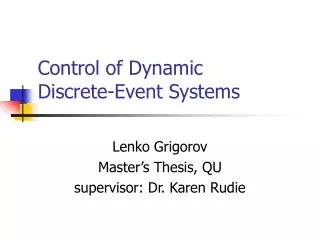
From Linear Systems to Discrete-Event Systems. W.M. Wonham Systems Control Group ECE Department University of Toronto Xidian University – Dec 2006 Update 2006.11.22. What is a Discrete-Event System?.

E N D
From Linear Systems to Discrete-Event Systems W.M. Wonham Systems Control Group ECE Department University of Toronto Xidian University – Dec 2006 Update 2006.11.22
What is a Discrete-Event System? • Structure with ‘states’ having duration in time, ‘events’ happening instantaneously and asynchronously. • States: machine is idle, is operating, is broken down, is under repair. • Events: machine starts work, breaks down, completes work or repair. • State space discrete in time and space. • State transitions ‘labeled’ by events.
Summary • Some history • Supervisory Control Theory (SCT) • Large systems (using IDDs) • Hierarchy • Extensions and Applications • Conclusions
Systems Control Concepts (c. 1980) • State space framework well-established: Controllability Observability Optimality (Quadratic, Lvarious, H) • Qualitative synthesis via controlled dynamic invariants • Use of geometric constructs and partial order: Controllability subspaces (c.s.) - supremal subspaces!
Discrete-Event Systems (c. 1980) • Practical problems • Programming languages for modeling & simulation • Queues, Markov chains • Petri nets • Boolean models • Formal languages • Process algebra (CSP, CCS)
Discrete-Event Systems Control (c.1980) • Control problems implicit in the literature (enforcement of resource constraints, synchronization, ...) But • Emphasis on modeling, simulation, verification • Little formalization of control synthesis • Absence of control-theoretic ideas • No standard model or approach to control
Needed (1980): DES Control Theory • System model Discrete in time and (usually) space Asynchronous (event-driven) Nondeterministic - support transitional choices • Amenable to formal control synthesis - exploit control concepts • Applicable: manufacturing, traffic, logistic,...
Proposed (1982):Supervisory Control Theory(Ramadge & Wonham) • Automaton representation - internal state descriptions for concrete modeling and computation • Language representation - external i/o descriptions for implementation-independent concept formulation • Simple control‘technology’
Community Response Anonymous Referees (1983-87) • Automatica “Automata have no place in control engineering.” Reject! • Mathematical Systems Theory • “Finite automata and regular languages are • nothing new at best and trivial at worst.” • Reject! • SIAM J. Control & Optimization • “So this is optimal control? Well...”Accept
Summary • Some history • Supervisory Control Theory (SCT) • Large systems (using IDDs) • Hierarchy • Extensions and Applications • Conclusions
Automaton controllable Idle MACH Down Wkg • Control Technology • = {, } {, } = con uncon uncontrollable SCT Base Model
0 10 13 11 1 2 12 TCTMACH MACH := (Q, , , q0, Qm) MACH = Create (MACH) >name:MACH ># states:3 {TCT Q := {0,1,2}, q0 := 0} >marker state(s): 0 {TCT Qm := {0}} > transitions:[0,11,1], [1,10,0], [1,12,2], [2,13,0] {TCT := {10, 11, 12, 13}, : Q Q transitions} > quit<Ret> {TCT files MACH.DES}
I W D SCT Languages • Closed and Marked Behaviors L(MACH) = all strings generable from initial state I = {, , , , , , …} = closed behavior of MACH Lm(MACH) = all generable strings hitting some marker state = {, , , …} = marked behavior of MACH prefix closure • _________ • Liveness (Nonblocking):Lm(MACH) = L(MACH)
Synchronous Product • Builds a more complex automaton with more complex language shared L(A1 A2) = P1-1L(A1) P2-1 L(A2) expressed bynatural projections Pi: (1 2)* i* (i = 1,2)
Transfer Line TL (Al-Jaar & Desrochers) 1 4 5 6 2 3 M1 B1 B2 TU M2 8 SCT Complex Plant • Complex plant = sync product of simplesubplants TL = M1 || M2 || TU
2, 8 2, 8 2,8 B1 3 3 3 4 B2 5 SCT Complex (Safety) Specification • Complex specification = sync product of partial specifications BUFFSPEC = B1 || B2
General Control Issues • Is there a control that enforces bothsafety, and liveness (nonblocking),and which is maximally permissive ? • If so, can its design be automated? • If so, with acceptable computingeffort?
SCT Synthesis - Problem E.g. for TL, let ConTL = ‘TL under control’ Must guarantee 1. Safety: Lm(ConTL) Lm(BUFFSPEC) 2. Liveness (nonblocking): Lm(ConTL) = L(ConTL) 3. Maximal permissiveness: Lm(ConTL) = maximum subject to safety and liveness
SCT Synthesis - Solution E.g. for TL: 1. Fundamental definition A sublanguage K Lm(TL) is controllable if __ K uncon L(TL) K “Once in K, you can’t skid out on an uncontrollable event.” 2. Fundamental result There exists a (unique)supremalcontrollable sublanguage Ksup Lm(TL) Lm(BUFFSPEC) Furthermore Ksup can be effectively computed.
* (all strings) Lm(TL) Lm(BUFFSPEC) Lm(TL) Lm(BUFFSPEC) optimization Ksup (optimal) K' K" (suboptimal) (no strings) SCT Synthesis Lattice
‘Monolithic’ SCT Implementation • Given TL and BUFFSPEC, compute Ksup Ksup= Lm(SUPER) SUPER = supcon (TL, BUFFSPEC) •Given SUPER, implement Ksup TL Ksup enable/disable events in con SUPER
TCT TRANSFER LINE (TL) M1 = Create (M1), M2 = Create (M2), TU = Create (TU) TL = Sync (M1, M2, TU) {synchronous product} B1 = Create (B1), B2 = Create (B2) BUFFSPEC = Sync (B1, B2) {synchronous product} SUPER (.DES) = SupCon (TL, BUFFSPEC) {optimization} SUPER (.DAT) = ConDat (TL, SUPER(.DES)) {control data} SIMSUP = SupReduce (TL, SUPER(.DES), SUPER(.DAT)) {supervisor reduction} SIMSUP (.DAT) = ConDat (TL, SIMSUP) {control data}
Summary • Some history • Supervisory Control Theory (SCT) • Large systems (using IDDs) • Hierarchy • Extensions and Applications • Conclusions
PLANT = sync (PLANT.1, … , PLANT.m) SPEC = sync (SPEC.1, … , SPEC.n) SUPER = supcon (PLANT, SPEC) State size of SUPER~ (Constant) m+n Exponential state space explosion ! ‘Extensional’ listing of ‘flat’ transition structures is impossible ! Large DES
What To Do ? • In state representations, retain product structurePLANT state vector x = [x1, ... , xm]SPEC state vector y = [y1, … , yn] • Express SUPER as a predicate Predsup (x, y, , x, y) = 0 or 1 • Algorithmize representation of Predsup using Integer Decision Diagrams (IDDs)
Root x1 0 1 2 Order! x2 0 1 0 0 1 1 f 1 0 1 0 0 0 Reduce! Root x1 0 2 1 IDD x2 0 0 1 f 1 0 Integer Decision Diagrams (IDDs) • IDDs represent functions on finite sets
Manufacturing Workcell (Barkaoui & Ben Abdallah 1995, Seidl 2000) Input 1 Output 2 Machine 2 Machine 1 Robot 1 Machine 4 Machine 3 Input 2 Output 1 Robot 2
Green Production Sequence (‘safety’ specification) M1 Robot 2 O1 I1 M3 Robot 1 Robot 1 M2 Red Production Sequence (‘safety’ specification) Robot 2 Robot 1 Robot 1 I2 M4 M2 O2 ?! Robot 1 Robot 1 M4 M2 M3 Workcell Control Issues Blocking! (prohibit by nonblocking ‘liveness’ spec’n)
Computing Effort vs. |Nodes| • Computing time ~ |Nodes|1.5 << |States| • Memory usage ~ |Nodes| K • For ‘loosely coupled’ practical systems |Nodes| ~ N K Cwhere N = number of system components (m+n)Kstate size of individual automataC= coupling coefficient 2 • |Nodes| linear (not exponential!)in N
{0,1}n state vector Control IDDs SUPER PLANT new event new enabled event set Supervisor Implementation
Summary • Some history • Supervisory Control Theory (SCT) • Large systems (using IDDs) • Hierarchy • Extensions and Applications • Conclusions
Manager (slow) scope Operator (fast) Architecture:Hierarchical Layering • Scope # subordinates • time horizon • bandwidth –1 • frequency –1 of significant events • Scope ratio (adjacent levels) 5:1 • e.g. 20,000 employees 7 levels
? plan = report (control command) Hierarchical Consistency plan HI MANAGER HI WORLD advise command report fb LO OPERATOR LO WORLD control
PLANThi T T* M (M) report command PLANTlo * L (L) report is modelled by : L T *, (L) =: M Report and Command -1 command is modelled by -1 : (M) (L)
sup M () M(M)(M) -1 sup L() L (L)(L) Achieving Hierarchical Consistency By design of T, arrange “ is an observer and preserves controllability” Then diagram commutes, giving hierarchical consistency
M1 B1 B2 TU M2 HierarchicalTransfer Line For hierarchical control, bring in manager’s hi-level alphabet Twith events , ', ... Event = ‘TU returns faulty workpiece for reworking’
Hierarchical Transfer Line –LO to HI
fail fail pass pass SPEC - HI fail fail pass SUPER - HI pass Hierarchical Transfer Line -HI-Level Synthesis
Summary • Some history • Supervisory Control Theory (SCT) • Large systems (using IDDs) • Hierarchy • Extensions and Applications • Conclusions
Extensions to Base Model • Forced (preemptive) events • Timed events (delays, deadlines, forcing) - Brandin, Saadatpoor • Liveness (= eventuality), temporal logic – infinite-string ( - languages) - Fusaoka,Thistle, Ramadge • Liveness (fairness, -calculus) - Thistle,Ziller • Algebraically hybrid (?) – X = Q1 ... Qk n m
Some Applications • Communication protocol specification (Rudie 1990) • Rapid thermal multiprocessor (Hoffmann 1991) • Robotic agents (Kosecka 1994) • AIP automated manufacturing system • (Brandin 1994, Leduc 2001, Ma 2003) • Telephonefeature interaction (Thistle 1995) • Chemical process control • (Sanchez 1996, Alsop 1996) • Truck dispatching (Blouin 2001) • Telephone directory assistance call center (Seidl 2004)
Conclusions • Achievements of SCT: * Syntheticand general * Resultscorrect by construction and computable for large systems * Modulararchitecture for management of complexity * Easy to teach and use (e.g. materials on Internet) • Challenges for SCT: • * How to interpret and modify controller structure (e.g. IDDs linear inequalities) ? • * How to find general laws of architecture ?