Download
1 / 30
300 likes | 416 Views
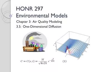
HONR 297 Environmental Models. Chapter 3: Air Quality Modeling 3.2: Physical Principles. Initial Assumptions. For our investigation of air quality models, we will focus on point sources of air pollution – the main reason is to allow us to work with simpler mathematical models.

E N D
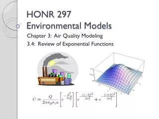
HONR 297Environmental Models Chapter 3: Air Quality Modeling 3.2: Physical Principles
Initial Assumptions • For our investigation of air quality models, we will focus on point sourcesof air pollution – the main reason is to allow us to work with simpler mathematical models. • We will also assume that the point sources are in a steady state, i.e. the amount of material being released from a point source doesn’t change over the time period we are considering. • A standard example of a point source in steady state to keep in mind is a smoke stack that is releasing a steady amount of smoke or gases at its top!
Smoke Stacks • Think of all the smoke stacks you have ever seen, ranging from large factory or power plant stacks to a single chimney on a house. • Essentially all such stacks are the same. • In this section, we will look at the various processes that affect the way smoke disperses once released. • With this in mind …
Smoke Stacks – Emissions Plume • What mental images do you have of the emissions plume from a smoke stack? • Let’s take a few moments to think about this …
Smoke Stacks – Emissions Plume • Does the plume • Go directly upward? • Turn to one side? • Spread out in the vertical direction? • Stay confined to a single limited level? • Climb higher and higher? • Move down towards the ground? • Do anything else?
Smoke Stacks – Emissions Plume • Sample plume behavior, from Hadlock, Figure 3.1, p. 62. Image Courtesy Charles Hadlock: Mathematical Modeling in the Environment
Smoke Stacks – Emissions Plume • Exhaust emitted from a smoke stack can take on many different patterns. • One big factor will be wind, but there are many others, as we will see. • Suppose we want to study plume behavior from an existing smoke stack or want to predict behavior for exhaust from a new building before it is built!
Mathematical Models • To make these types of predictions about plume behavior, we can use mathematical models that take into account factors such as • Nature of the proposed (or existing) site. • Historical or typical weather patterns in the area. • Physical characteristics of the smoke stack. • Etc. • This is what is done by both plant/site designers and regulatory agencies!
Pollutant Dispersal Processes • The key physical processes that control the way pollutants disperse into the atmosphere can be classified as follows: • The propensity of gaseous materials to move from areas of higher concentration to areas of lower concentration by means of a simple diffusion process. • The patterns of movement of the surrounding air, including both horizontal movement (wind) and vertical movement. • The physical characteristics of the exhaust gases themselves, such as temperature, momentum, and perhaps other properties. • Other aspects of the surroundings, such as special topographic features or changes in elevation.
Diffusion • What happens if a small amount of perfume is placed on a cloth or sprayed in room? • Shortly thereafter, the perfume will have spread throughout the room. • The reason is that the gas molecules generated by evaporation of the perfume start out at a high concentration near the point of origin and tend to spread out to areas of lower concentration, eventually permeating the whole room. • The same happens if gasoline is spilled – the gasoline vapors will move from the area of higher concentration near the spill to areas of lower concentration throughout the room. • Another example is a lump of sugar in a cup of coffee or tea – dissolved sugar molecules will gradually spread out throughout the liquid, even without any stirring – again, the sugar molecules are moving from areas of higher concentration of sugar to areas of lower concentration. • All of these situations are examples of a process known as diffusion!
Diffusion • From Wikipedia: • Diffusion is one of several transport phenomena that occur in nature. A distinguishing feature of diffusion is that it results in mixing or mass transport without requiring bulk motion. In Latin [the] word "diffundere" means "to spread out". • (Wikipedia link) (YouTube video) • YouTube Video – Diffusion • Diffusion is caused by kinetic energy (i.e. energy due to motion) present in individual molecules which causes them to bounce around in random patterns until they are more evenly distributed – this type of motion is often referred to as a random walk. • This process is similar to shuffling a deck of cards – if one starts with all hearts together in one place and shuffles the cards a number of times (a randomizing process), the hearts will eventually be mixed into the deck in a more uniform and spread out fashion.
Three-Dimensional Diffusion • We can think of diffusion as a process that is three – dimensional, two – dimensional, or even one – dimensional, depending on a given physical situation! • Using the perfume example, imagine a puff of perfume is sprayed in the center of a room, as shown to the right (Figure 3.2 of Hadlock, p. 63). Image Courtesy Charles Hadlock: Mathematical Modeling in the Environment
Three-Dimensional Diffusion • Initially, all of the perfume is concentrated near the center of the room. • As time progresses, the perfume molecules will spread out in a uniform fashion, in all directions! • The driving mechanism is the kinetic energy in the perfume molecules, spreading out via random walks! Image Courtesy Charles Hadlock: Mathematical Modeling in the Environment
Three-Dimensional Diffusion • If we measure the concentration in the x-, y-, or z- direction at times t1, t2, and t3, where t1 < t2 < t3, we will find that the concentration (as a function of distance from the center of the room will have shapes similar to those given in Hadlock as Figure 3.3 on p. 64. Image Courtesy Charles Hadlock: Mathematical Modeling in the Environment
Two-Dimensional Diffusion • Diffusion can also occur in two dimensions – imagine for example a drop of ink placed in the center of a white handkerchief or a thin layer of gelatin. • Again, the ink molecules are moving from an area of higher concentration to lower concentration via random walks! • Two dimensional diffusion can also be used to model perfume sprayed at the center of a “low-ceilinged room” or a uniform vertical column of perfume in the middle of a room, as shown to the right (Figure 3.4 in Hadlock, p. 65). Image Courtesy Charles Hadlock: Mathematical Modeling in the Environment
Two-Dimensional Diffusion • For each of these cases, the idea to keep in mind is that every vertical level is assumed to be identical to the levels above and below – there is no difference in concentration as we move vertically, only as we move horizontally does the concentration change! • In this case, we’d expect concentration graphs similar to those in Figure 3.3, at instances in time, measured as a function of distance from the source, as we move in the x- or y-direction! • What would the concentration look like as we move in the z-direction from the center in the second situation, at instances in time? • Constant concentration, which will reduce over time … • Note: In the second situation shown to the right, we call the column of perfume a line source. Image Courtesy Charles Hadlock: Mathematical Modeling in the Environment
One-Dimensional Diffusion • If we spray perfume in a tube filled with air or have a situation in which a wall running down the middle of a room has been painted, we can model the process by which the perfume, or paint fumes spread out as one-dimensional diffusion. • In this case, at any instant in time, concentration of the perfume or paint smell depends only on the distance along the tube from the center or perpendicular distance from the wall. • Hadlock provides figures to illustrate this – see Figure 3.5 on p. 66. • In this case, we’d expect concentration graphs similar to those in Figure 3.3, at instances in time, measured as a function of distance from the source, as we move in the x- direction! • In the y- or z- direction, the concentration would be constant at any given instant in time! • Note: in this case, we call the wall of paint a “planar source”. Image Courtesy Charles Hadlock: Mathematical Modeling in the Environment
Air Movement • So far, we’ve been discussing the first physical process that controls the way pollutants disperse in the atmosphere, namely, • The propensity of gaseous materials to move from areas of higher concentration to areas of lower concentration, which is achieved via diffusion! • The second factor we need to look at when dealing with pollutant dispersal in the air is the movement of the air itself!
Air Movement • Question: • Suppose we live one mile from a power plant and the wind is blowing directly from the power plant towards our home. • Further, suppose there is some level of contaminants in the air near our house as a result. • What would happen if we had the same situation, but the wind is blowing twice as hard? • Think about this for a few minutes …
Air Movement • Possible answers: • The wind is harder, so the air moves faster, which implies that pollutants travel to our house more quickly, with less time to diffuse, so the pollution concentration levels near our house increase. • The wind is blowing harder, so the air is stirred up more, which increases the diffusion rate, so the pollution concentration levels near our house decrease.
Air Movement – Wind Speed • Wind speed is not constant at all heights above the ground. • Friction of the air mass along the ground causes air near the earth’s surface to move more slowly than air higher up. • This is illustrated in Figure 3.6, p. 67 of Hadlock, shown above – longer arrows indicate greater wind speed. • This difference in wind speed as we move vertically upwards from the earth’s surface, known as a “wind-speed gradient”, causes mixing between adjacent layers of air, with a net result of vertical transport of pollutants! Image Courtesy Charles Hadlock: Mathematical Modeling in the Environment
Air Movement – Solar Insolation • Solar insolation (i.e. sunlight) warms the ground, which in turn warms the air above it. • This makes the air near the earth’s surface less dense, causing it to rise (similar to how a hot air balloon works), as in Hadlock’s Figure 3.7 above. • As the warmer air rises, air moves in from the sides or above, again causing vertical mixing of air, hence vertical mixing of pollutants if present! Image Courtesy Charles Hadlock: Mathematical Modeling in the Environment
Exhaust Gas Characteristics • A third factor we must consider when working with dispersal of pollutants in the air is physical characteristics of the exhaust gases, themselves! • Exhaust gas is hot, so it will rise! • Exhaust gases will be moving at a high velocity, so they exit rapidly from the top of a smoke stack and continue to move upward vertically for some distance (they have momentum), until they mix with or are slowed down by the surrounding air mass. • The net effect of hot gas and momentum is that initially the exhaust gases move upwards in a column, so we can think of this as an imaginary extension of the stack height, possibly from two to ten times the actual stack height! • See Hadlock, Figure 3.8 shown above. Image Courtesy Charles Hadlock: Mathematical Modeling in the Environment
Surface Characteristics • Finally, a factor that contributes to the dispersal of pollution in the air is characteristics of the earth’s surface, including • Changes in elevation (topography), which can cause deflection of exhaust plumes. • Surface roughness (trees vs. buildings vs. open fields vs. water), which can cause vertical mixing in a fashion similar to that discussed above for wind velocity gradients.
Surface Characteristics Images Courtesy Charles Hadlock: Mathematical Modeling in the Environment
Summary • In summary, the four main factors that affect dispersion of air pollutants are • Tendency of pollutants to Diffuse, causing movement from high to low concentration • Air Movement and Mixing • Exhaust Gas Characteristics • Surface Characteristics • Of these, the first and second will be the most important for our models. • It will turn out that the third and fourth factors can be incorporated into the models we will use in a simple fashion.
Stability • Finally, for our mathematical models, we will need some additional background material related to air movement and mixing, namely the concept of stability. • Definition: • We say an air mass is stable if there is relatively little vertical mixing per unit of horizontal distance traveled. • An air mass is said to be unstable if the amount of vertical mixing per unit of horizontal distance is relatively high. • We expect a plume of exhaust gas to disperse less in stable atmospheric conditions and disperse more in unstable atmospheric conditions! • Thus, we can think of a stable air mass as corresponding to a stable plume and an unstable air mass as corresponding to an unstable plume! • See Hadlock, Figure 3.11 at right. Image Courtesy Charles Hadlock: Mathematical Modeling in the Environment
Stability • What characteristics might affect plume stability (think of what might affect air stability in general)? • Wind speed. • Solar insolation. Image Courtesy Charles Hadlock: Mathematical Modeling in the Environment
Pasquill-Gifford Stability Categories • Meteorologists have studied various combinations of atmospheric conditions and have developed a scheme for classifying air stability! • The scheme (which is used by industry and regulatory agencies) is summarized in Table 3.1 on p. 71 of Hadlock. • Air stability is classified from A (most unstable) to F (most stable), as a function of • Wind speed (measured 10 meters above the ground). • Incoming solar radiation (see table for details). • Cloud cover at night (see table for details).
Resources • Wikipedia (diffusion definition) • http://en.wikipedia.org/wiki/Diffusion • You Tube Videos • http://www.youtube.com/watch?v=c_FZy6XVDQU • http://www.youtube.com/watch?v=6zysNwl6Zuo • http://www.youtube.com/watch?v=_oLPBnhOCjM • Charles Hadlock, Mathematical Modeling in the Environment, Section 3.2 • Figures 3.1 – 3.11 used with permission from the publisher (MAA).