Download
1 / 35
350 likes | 450 Views
Geophysical wave interactions in turbulent magnetofluids. Shane R. Keating University of California San Diego Collaborators: Patrick H. Diamond (UCSD) L. J. Silvers (Cambridge) Keating & Diamond (Jan 2008) J. Fluid Mech. 595

E N D
Geophysical wave interactions in turbulent magnetofluids Shane R. Keating University of California San Diego Collaborators: Patrick H. Diamond (UCSD) L. J. Silvers (Cambridge) Keating & Diamond (Jan 2008) J. Fluid Mech. 595 Keating & Diamond (Nov 2007) Phys. Rev. Lett. 99 Keating, Silvers & Diamond (Submitted) Astrophys. J. Lett. March 12, 2008 Courant Institute for Mathematical Sciences
In a nutshell… • Turbulent resistivity is “quenched” below its kinematic value by an Rem-dependent factor in 2D MHD turbulence. • Mean-field electrodynamics offers little insight into the physical origin of small-scale irreversibility, relying upon unconstrained assumptions and a free parameter (). … Borrowing some ideas from geophysical fluid dynamics… • Introduce a simple extension of the theory which does possess an unambiguous source of irreversibility: three-wave resonances. • Rigorously calculate the spatial transport of magnetic potential induced by wave interactions. This flux is manifestly independent of Rem.
Statement of the problem Statement of the problem: How fast are magnetic fields dissipated in 2D turbulence? Nomenclature: Magnetic potential: B = r A £ey Induction equation: t A + u¢r A = r2 A where A(x, z, t) = hAi+ a(x, z, t) Introduce turbulent flux: hu ai = - TrhAi then thAi2 = 2 ( + T)hBi2
Resistivity quenching in 2D MHD I • In the presence of even a weak mean magnetic field, the dissipation of magnetic fields is strongly suppressed below its kinematic value in 2D MHD: Cattaneo & Vainshtein (1991) Magnetic energy density (normalized) Increasing initial magnetic field strength Time
Resistivity quenching in 2D MHD II • Quasi-linear theory gives (Gruzinov & Diamond 1994): kin¼ U L • kinematic resistivity • Initial magnetic energy in units of the kinetic energy • Magnetic Reynolds number X2 = B02 / h u2i Rem = U L / c • Implicit assumption: the spatial transport of magnetic • potential is suppressed, not the turbulence intensity…
Keating, Silvers & Diamond (2008) Ln normalized cross-phase Ln square of initial field Resistivity quenching in 2D MHD III • Is the quench due to a suppression of the spatial transport of magnetic potential or a suppression of the turbulence itself? • Useful diagnostic: the normalized cross-phase • Quench then becomes
Quenching: Competing couplings/cascades • Physically, expect: turbulence strains and chops up a scalar field, generating small-scale structure magnetic potential tends to coalesce on large scales: Ais not passive forward cascade of A2 to small scales inverse cascade of A2 to large scales “positive viscosity” effect “negative viscosity” effect
here be dragons Turbulent resistivity: Quenching: Closure calculation • EDQNM calculation of the vertical flux of magnetic potential A (Gruzinov & Diamond 1994, 1996) • Quasi-linear closure: • Quasi-linear response:
The key question • These closure calculations offer no insight into the detailed microphysics of resistivity quenching because the microphysics has been parametrized by , a free parameter in EDQNM / quasi-linear closures. What sets the timescale τ? • Motivated to explore extensions of the theory for which the correlation time is unambiguous.
“Wavy MHD” in 2D Coriolis force buoyancy • MHD + additional body forces: Rossby waves internal waves • Large-scale eddies dispersive waves: “Wavy MHD” = MHD + dispersive waves • (c.f. Moffatt (1970, 1972) and others) • When the wave-slope < 1, wave turbulence theory is applicable. • Origin of irreversibility is in three-wave resonances, which are present even in the absence of c
latitudinal gradient in locally vertical component of planetary vorticity mean magnetic field Illustration 1: plane MHD I • Quasigeostrophic MHD turbulence in a rotating spherical shell • “Minimal model” of solar tachocline turbulence (Diamond et al. 2007): MHD turbulence on a plane • symmetry between left and right is broken by N
l* Illustration 1: plane MHD II • modifies the linear modes: Alfven wave Rossby wave dominant for small scales (large k) dominant for large scales (small k) non-dispersive dispersive small scales large scales
buoyancy term mean magnetic field density gradient Illustration 2: stratified MHD I • 2D MHD in the presence of stable stratification • additional dynamical field: density • Boussinesq approximation: appears only in buoyancy term • Minimal model of stellar interior just below solar tachocline N
Brunt-Vaisala frequency l* Illustration 2: stratified MHD II • stratification modifies the linear modes: Alfven wave Internal gravity wave dominant for small scales (large k) dominant for large scales (small k) non-dispersive dispersive small scales large scales
stable unstable Wave turbulence theory • describes the slow transfer of energy among a triad of waves satisfying the resonance conditions: • analogous to the free asymmetric top (I3 > I2 > I1) Landau & Lifschitz, Mechanics, 1960 • for an ensemble of triads, origin of irreversibility is chaos induced by multiple overlapping wave resonances
Wave turbulence theory: validity • Wave turbulence theory requires a broad spectrum of dispersive, weakly interacting waves
Wave turbulence theory: validity • Wave turbulence theory requires a broad spectrumof dispersive, weakly interacting waves • broad enough for triad to remain coherent during interaction
Wave turbulence theory: validity • Wave turbulence theory requires a broad spectrum of dispersive, weakly interacting waves • broad enough for triad to remain coherent during interaction • resonance manifold is empty for non-dispersive waves
Wave turbulence theory: validity • Wave turbulence theory requires a broad spectrum of dispersive, weakly interactingwaves • turbulent decorrelation doesn’t wash out wave interactions: • broad enough for triad to remain coherent during interaction • resonance manifold is empty for non-dispersive waves < 1 • for dispersive waves, this is unity for a cross-over scale:
Strong turbulence Weak turbulence Dispersive Non-dispersive I. Alvenic Range II. Intermediate Range III. Wavy Range Spectral ranges Vrms Horizontal phase velocity (vph,x) B0 L* l* Scale (k-1)
I. Alvenic Range II. Intermediate Range III. Wavy Range dispersive waves are washed out by turbulence molecular diffusion strongly interacting eddys and Alfven waves molecular diffusion waves are dispersive and weakly interacting molecular diffusion; nonlinear wave interactions character of turbulence sources of irreversibility Spectral regimes
The wavy regime • Within the wavy range the turbulent resistivity can be expanded in powers of the small parameter: Lowest order contribution is tied to c and so will depend upon Rm, Re, Pm… At higher order, nonlinear wave interactions make Rm-independent contribution • Overall turbulent resistivity has twoasymptotic parameters: Rm and wave-slope
Linear response Response to wave interactions Flux due to molecular collisions Flux due to wave-wave interactions The wave-interaction-driven flux I • Calculate the flux of A due to wave-interactions:
The wave-interaction-driven flux II • Expand A in powers of the wave-slope = k < 1 • First contribution to wave-interaction-driven flux is O(4) • Formal solution:
The wave-interaction-driven flux III • The flux driven by wave interactions is calculated to fourth order in the wave-slope • This is the same order as in wave-kinetic theory; however, we are interested in spatial transport rather than spectral transfer coupling coefficient fourth order in wave-slope geometrical factor §= Re i (’ + ’’ §k’ + k’’ + i 0+)-1 = (’ + ’’ §k’ + k’’) Resonance condition • Response time:
Irreversibility • Within the wavy range, origin of irreversibility is chaos induced by overlapping wave resonances • triads with one short, almost vertical leg dominate the coupling coefficient • “induced diffusion” triad class (McComas & Bretherton 1977) • short leg acts as a large-scale adiabatic straining field on other two modes • directly analogous to wave-particle resonances in a Vlasov plasma • For this triad class there exists a rigorous and transparent route to irreversibility based upon ray chaos
Conclusions • Within the wavy range, the origin of irreversibility is unambiguous: ray chaos induced by overlapping resonances • In the presence of dispersive waves, T does not decay asymptotically as Rm-1 for large magnetic Reynolds number • The presence of an additional restoring force can actually increase the transport of magnetic potential in 2D MHD • If so, concerns about resistivity quenching in real magnetofluids may be moot.
A useful analogy I • Nonlinear wave-particle interactions in a Vlasov plasma: • Diffusive flux of particles in velocity space can be expanded in powers of |Ek,|2 • Second-order flux driven by interaction between electron (v) and plasma wave (k,): • Fourth-order flux driven by interaction between electron (v) interacting with beating of two plasma waves (k+k’, + ’):
Fourth-order flux ~ Second-order flux ~ A useful analogy II
NL wave interactions: Basic paradigms I • Free asymmetric top (I3 > I2 > I1) Landau & Lifschitz, Mechanics, 1960 perturbations about stable axes are localized perturbations about unstable axis wander around entire ellipsoid • Energy is slowly transferred from x2 to x1 or x3 • However, motion is ultimately reversible
NL wave interactions: Basic paradigms II • Three nonlinearly coupled oscillators • Formally equivalent to the asymmetric top • Assuming weak coupling: Ai(t) are slow functions of t • Equations of motion will be dominated by slow, secular drive of one oscillator on the other two if oscillator frequencies satisfy “three-wave resonance” condition: • In this case, equations governing amplitudes Ai(t) are: • As in the asymmetric top, one of the modes can pump energy into the other two at a rate: Basic timescale for nonlinear transfer of energy d ~ • However, also like the asymmetric top, such transfer is reversible!
NL wave interactions: Basic paradigms III • Wave turbulence theory: • ensemble of many wave triads (statistical theory) • infinite moment hierarchy (closure problem) • key timescales: • three-wave mismatch • triad lifetime : tied to dispersion • nonlinear transfer rate • expand in small parameter (turbulentintensity) Wave turbulence requires a broad spectrum of dispersive waves • Origin of irreversibility: • Mechanically: Random phase approximation • moment hierarchy is truncated • Physically: ray chaos induced by resonance overlap