Download
1 / 25
270 likes | 600 Views
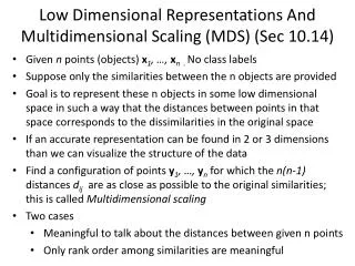
Modern Multidimensional Scaling 8. A Majorization Algorithm for Solving MDS. 2009-02-25 숭실대학교 기계학습 연구실 주상훈 shju@ml.ssu.ac.kr. The Stress Function for MDS. Six definitions n denotes the number of empirical objects. Stimuli, variables, items, questions, and so on, depending on context

E N D
Modern Multidimensional Scaling8. A Majorization Algorithm for Solving MDS 2009-02-25 숭실대학교 기계학습 연구실 주상훈 shju@ml.ssu.ac.kr
The Stress Function for MDS • Six definitions • n denotes the number of empirical objects. • Stimuli, variables, items, questions, and so on, depending on context • If an observation has been made for a pair of objects i and j, a proximity value pij is given. • proximity – both similarity and dissimilarity • missing value – If pij is undefined • Dissimilarity is a proximity that indicates how dissimilar two objects are. • X denotes • (a) a point configuration (i.e., a set of n points in m-dimensional space) • (b) the n*m matrix of the coordinates of the n points relative to m Cartesian coordinate axes. • The Euclidean distance between any two points i and j in X is the length of a straight line connection pointsiand j in X. • The term f(pij) denotes a mapping of pij, that is the number assigned to pij according to rule f. • We define an error of representation by • eij 2 = (dij - δij) 2 • The final version of raw stress • σr(X) = Σi<jwij(dij(X) - δij)2.
Mathematical Excursus : Differentiation • f(x) = y = 0.3x4 - 2x3 + 3x2 + 5 • Slope zero = B, C, E • Local minimum = B, Global minimum = E, Local maximum = C • There is no global maximum. • If we determine the tangent for each point on the graph, it becomes evident that they are horizontal lines at the extrema of the displayed potion of the graph
The Slope of a Function - I • The symbol dy/dx denotes the resulting limit of this operation. Note carefully that the limit dy/dx is not generated by setting Δx = 0, but by approximating Δx = 0 arbitrary closely. • This function is giving the slope of the tangents or the growth rate of y relative to x at each point P. (Be called the derivative of y = f(x), usually denoted by y’)
The Slope of a Function - II • The derivative of y = x2can be found by considering the slope of the tangent at point P. • y‘=2x, the slope of the tangent at each point is simply twice its x-coordinate. • For x=5, say, we obtain the slope dy/dx = 10, which means that y=x2grows at this point at the rate of 10y-units per 1 x-unit.
Finding the Minimum of a Function • f(x) = y = 0.3x4 - 2x3 + 3x2 + 5 • We find by rules 1,4, and 8: • dy/dx = (0.3)(4)x3 - (2)(3)x2 + (3)(2)x = 1.2x3 – 6x2 + 6x • 1.2x3 – 6x2 + 6x = 0 • (x)(1.2x2 - 6x + 6) = 0 • x1 = 0, x2 = 3.618, x3 = 1.382 (correspond to points B, C, and E in graph.)
Second- and Higher-Order Derivatives • The derivative of a function y = f(x) is itself a function of x, y’ = f’ (x). • One therefore can ask for the derivative of y’, y’’= f’’(x), the derivative of y’’, and so on. • First Example, • y = x3 • y' = 3x2 • That is, at any point x, the cubic function grows by the factor 3x2. • y'' = 3*2x = 6x • This means that the rate of change of the growth rate also depends on x: it is 6 times the value of x. So, with large x values, the growth of x3 “accelerates” quite a bit. • Second Example, • y = x1/2, x > 0 • y'' = f ' (1/2* x-1/2) = (-1/4) * x-3/2 = -1/(4x3/2) • y' shows that this function has a positive slope at any point x, and y'' indicates that this slope decrease as x becomes larger. • The second derivative is useful to answer the question of whether a stationary point is a minimum or a maximum.
Partial Derivatives and Matrix Traces • We often deal with functions that have more than one variable. • Such functions are called functions with several variables, multivariable functions, vector functions, or functions with many arguments. • E.g., raw Stress, σr(X) • Because we attempt to minimize this function over every single one of its n*m coordinates, we naturally encounter the question of how to find the derivative of multivariable functions. • The answer is simple • such functions have as many derivatives as they have arguments, and the derivative for each argument xi is found by holding all other variables fixed and differentiating the function with respect to xi as usual. • Example, • The derivative of the function f(x,y,z) = x2y + y2z + z2x with respect to variable y is x2 + 2yz, using rules 4 and 8 of Table 8.1 and treating z2x as a “constant” (i.e., as not dependent on y) • The derivative to one argument of a function of several variables is called the partial derivative. The vector of partial derivatives is called the gradient vector.
Partial Derivatives and Matrix Traces • Here, the constants are collected in the matrix A, the variables in X. Suppose that we want to find the partial derivative of the linear function f(X) with respect to the matrix X.
Minimizing a Function by Iterative Majorization • Iterative Majorization • For finding the minimum of a function f(x). • A set of computational rules that are usually applied repeatedly, where the previous estimate is used as input for the next cycle of computations which outputs a better estimate. • The central idea of the majorization method is to replace iteratively the original complicated function f(x) by an auxiliary function g(x,z), where z in g(x,z) is some fixed value. • The functions g has to meet the following requirements to call g(x,z) a majorizing function of f(x) • The auxiliary function g(x,z) should be simpler to minimize than f(x). • The original function must always be smaller than or at most equal to the auxiliary function; that is, f(x) <= g(x,z) • The auxiliary function should touch the surface at the so-called supporting point z; that is, f(z) = g(z,z)
Principles of Majorization • F(x*) <= g(x*,z) <= g(z,z) = f(z) • The iterative majorization algorithm is given by • Set z = z0, where z0 is a starting value. • Find update xu for which g(xu,z) <= g(z,z) • If f(z) – f(xu) < ε, then stop (ε is a small positive constant.) • Set z = xu and go to 2.
Linear and Quadratic Majorization - Linear • Two class of majorization: linear and quadratic. • An example of the concave function f(x) = x1/2 • It is always possible to have a straight line defined by g(x,z) = ax+b (with a and b dependent on z) such that g(x,z) touches the function f(x) at x = z, and elsewhere the line defined by g(x,z) is above the graph of f(x). • Clearly, g(x,z) = ax+b is a linear function in x. Therefore, we call this type of majorization linear majorization. • Any concave function f(x) can be majorized by a linear function g(x,z) at any point z.
Linear and Quadratic Majorization - Quadratic • The second class of functions that can be easily majorized is characterized by a bounded second derivative. • This type of majorization can be applied if the function f(x) can be majorized by g(x,z) = a(z)x2 – b(z)x + c(z), with a(z) > 0, and a(z), b(z), and c(z) functions of z, but not of x. • We call this type of majorization quadratic majorization.
Example: Majorizing the Median - I • How can we majorize f(x)? • Begin by nothing that g(x,z) = |z|/2 + x2 / |2z|majorizes|x| • Three requirements • g(x,z)is simple function because it is quadratic in x. • we have f(x)<= g(x,z)for all x and fixed z. • This can be seen by using inequality (|x| - |z|)2 >= 0 • There must be equality in the supporting point; that is, f(z) = g(x,z)
Example: Majorizing the Median - II • The minimum of g(x,x0) is attained at x1≒ 6.49. • The next step in the majorization algorithm is to declare x1 to be the next supporting point, to compute g(x, x1) and find its minimum x2, and so on. After some iterations, we find that 4 is the minimum for f(x).
Visualizing the Majorization Algorithm for MDS - I • We see, for example, that the Dow Jones(dj) and Standard & Poors(sp) indices correlated highly, because they are very close together. • We also see that the European indices (brus, dax, vec, cbs, ftse, milan, and madrid) are reasonably similar. • The Asian markets (hs, nikkei, taiwan, and sing) do not seem to correlate highly among one another as they are lying at quite some distance from one another. • To see how the iterative majorization algorithm for MDS works, • Consider the situation where the coordinates of all stock indices are kept fixed at the position except for the point nikkei.
Majoring Stress • So far, we have discussed the principle of iterative majorization for functions of one variable x only. • The same idea can be applied to functions that have several variables. As long as the majorizing inequalities hold, iterative majorization can be used to minimize a function of many variables. • Components of the Stress Function • The first part, ηδ2, is only dependent on the fixed weights wij and the fixed dissimilarities δij, not dependent on X; so ηδ2 is constant. • The second part, η2(X), is a weighted sum of the squared distances dij2(X) • The third part, -2ρ(X), is a weighted sum of “plain” distances dij(X).
A Compact Expression for the Sum of Squared Distances • We first look at η2(X), which is a sum of the squared distances. • For the moment, we consider only one squared distance dij2(X). • xa be column a of the coordinate matrix X. • ei be the i-th column of identity matrix I. • If n=4, i=1, and j=3 then ei’ = [1 0 0 0], ej’ = [0 0 1 0], so that (ei – ej)’ = [1 0 -1 0]. But this means that xia – xja = (ei – ej)’ xa • The matrix Aij is simply a matrix with aii=ajj=1, aij=aji=-1, and all other elements zero. • In general, vij = -wij, if i≠j and vii = Σj=1, j=inwij for the diagonal elements of V. • * Furthermore, η2(X) is a quadratic function in X, which is easy to handle
Majorizing Minus a Weighted Sum of Distances • We now switch to-ρ(X), which is minus a weighted sum of the distance; that is, • To obtain a majorizing inequality for –dij(X), we use the Cauchy-Schwarz inequality, • If we substitute pa by (xia – xja) and qa by (zia-zja) • With equality if Z=X. Dividing both sides by dij(Z) and multiplying by -1 gives • Proceeding as in previous page, a simple matrix expression is obtained: • Combining (8.21) and (8.22), multiplying by wijδij, and summing over i < j gives • Because equality occurs if Z=X, we have obtained the majorization inequality • Thus, -ρ(X) can be majorized by the function –tr X’B(Z)Z, which is linear function in X.
The SMACOF Algorithm for Majorizing Stress - I • Combining two previous equations give us the majorization inequality for the Stress function; that is, • Thus τ(X,Z) is a simple majorization function of Stress that is quadratic in X. • Its minimum can be obtained analytically by setting the derivative of τ(X,Z) equal to zero; that is • so that VX = B(Z)Z. • If all wij =1, then V+ = n-1J with J the centering matrix I-n-111’, so that the update simplifies to (Guttman transform)
An Illustration of Majorizing Stress - I • Assume that all wij = 1 • The dissimilarities • The starting configuration X[0] = Z and their distances, • The first step is to compute σr(X[0]) = 34.29899413, then we compute the first update Xu by the Guttman transform.
An Illustration of Majorizing Stress - II • The next step is to set X[1] = Xu and compute σr (X[1]) = 0.58367883, which conclude the first iteration. • The difference of σr (X[0]) and σr (X[1]) is large, so it make sense to continue the iterations. • The second update is • With σr (X[2]) = 0.12738894. We continue the iterations until the difference in subsequent Stress is less than 10-6. • After 35 iterations, the convergence criterion was reached with configuration


![What is Multidimensional Scaling [MDS] ?](https://cdn2.slideserve.com/4259744/what-is-multidimensional-scaling-mds-dt.jpg)


![What is Multidimensional Scaling [MDS] ?](https://cdn5.slideserve.com/9558171/what-is-multidimensional-scaling-mds-dt.jpg)