Download

1 / 26
270 likes | 282 Views
PHL - 541. Non-parametric Procedures. By Dr. Sabry Attia Professor of Pharmacology and Toxicology. Test of Significance: General Purpose.

E N D
PHL - 541 Non-parametric Procedures By Dr. Sabry Attia Professor of Pharmacology and Toxicology
Test of Significance: General Purpose The idea of significance testing.If we have a basic knowledge of the underlying distribution of a variable, then we can make predictions about how, in repeated samples of equal size, this particular statistic will "behave," that is, how it is distributed. Normal distribution (Gaussian distribution) of variables. • About 68 % of values drawn from a normal distribution are within one SD, σ > 0 away from the mean μ. • About 95 % of the values are within two SD. • About 99.7 % lie within three SD. • This is known as the 68-95-99.7 Sigma rule. Are most variables normally distributed? • Income in the population. • Incidence rates of rare diseases. • Heights in different cities. • Number of car accidents,,,,,,,,,,,,, Example: If we draw 100 random samples of 100 adults each from the general population, and compute the mean height in each sample, then the distribution of the standardized means across samples will likely approximate the normal distribution (Student's t distribution with 99 df). Now imagine that we take an additional sample in a particular city ("X") where we believe that people are taller than the average population. If the mean height in that sample falls outside the upper 95% tail area of the t distribution then we conclude that, indeed, the people of X city are taller than the average population.
Test of significance: General Purpose Sample size: Large enough or Very small. If very small, then those tests based on the assumption can be used only if we are sure that the variable is normally distributed, and there is no way to test this assumption if the sample is small (<5, unpaired). Measurement Scales: • Interval variables allow us not only to rank order the items that are measured, but also to quantify and compare the sizes of differences between them. For example, temperature, as measured in degrees Fahrenheit or Celsius, represent an interval scale. We can say that a temperature of 40 degrees is higher than a temperature of 30 degrees, and that an increase from 20 to 40 degrees is twice as much as an increase from 30 to 40 degrees. • Ratio variables are very similar to interval variables. Most statistical data analysis procedures do not distinguish between the interval and ratio properties of the measurement scales. • Nominalvariables (qualitative). For example, we can say the two individuals are different in terms of variable A (e.g., they are of different gender, colour, city, race etc.), but we cannot say which one "has more" of the quality represented by the variable. • Ordinal variables allow us to rank order the items we measure in terms of which has less and which has more of the quality represented by the variable, but still they do not allow us to say "how much more". Examples; good-better-best, upper-middle-lower.
Alternatives of Parametric and Nonparametric Methods Basically, there is at least one nonparametric equivalent for each parametric general type of test. In general, these tests fall into the following categories: Tests of differences between groups (independent samples); • t-test for independent samples alternatives the Mann-Whitney U test. • ANOVA alternatives Kruskal-Wallis analysis of ranks. Tests of differences between variables (dependent samples); • t-test for dependent samples alternatives Sign test and Wilcoxon's matched pairs test or McNemar's Chi-square (If the variables of interest are dichotomous in nature (i.e., "pass" vs. "no pass"). • Repeated measures ANOVA alternatives Friedman's two-way analysis of variance and Cochran Q test (if the variable was measured in terms of categories, e.g., "passed" vs. "failed"). Tests of relationships between variables. Correlation coefficient equivalents to Spearman R, Kendall Tau, Coefficient Gamma,Chi-square test, the Phi coefficient, and the Fisher exact test. If the two variables of interest are categorical in nature (e.g., "passed" vs. "failed" by "male" vs. "female")
When to Use Which Method? • It is not easy to give simple advice concerning the use of nonparametric procedures. • Each nonparametric procedure has its peculiar sensitivities and blind spots. • In general, if the result of a study is important (e.g., does a very expensive and painful drug therapy help people get better?), then it is always useful to run different nonparametric tests; should discrepancies in the results occur dependent on which test is used, one should try to understand why some tests give different results. • On the other hand, nonparametric statistics are less statistically powerful (less sensitive) than their parametric counterparts, and if it is important to detect even small effects one should be very careful in the choice of a test statistic.
Nonparametric Methods: Mann-Whitney U or Wilcoxon rank sum test (MWW) Frank Wilcoxon (1892-1965) • Mann-Whitney U test is one of the best-known non-parametric significance test and is included in most modern statistical packages. It is also easily calculated by hand for small samples. • It was proposed initially by Frank Wilcoxon in 1945 for equal sample sizes, and extended to arbitrary (random) sample sizes and in other ways by Mann and Whitney (1947). • MWW test is practically identical to performing an ordinary parametric two-sample t test on the data after ranking over the combined samples. They are excellent alternatives to the t test if your data are significantly skewed. • MWW test tests for differences in medians and for chances of obtaining greater observations in one population versus the other. • The null hypothesisin the MWW test is that both populations have the same probability of exceeding each other. i.e. no difference in the two population distributions. • The alternative hypothesisis that the variable in one population is stochastically greater. • The test involves the calculation of a statistic, usually called U (the sum of ranks), whose distribution under the null hypothesis is known. In the case of small samples, the distribution is tabulated, but for sample sizes above ~ 20 there is a good approximation using the normal distribution methods.
Nonparametric Methods: Mann-Whitney U test Assumptions for Mann-Whitney U Test: • The two samples under investigation in the test are independent of each other and the observations within each sample are independent. • The observations are ordinal or continuous measurements (i.e., for any two observations, one can at least say, whether they are equal or, if not, which one is greater). Data types that can be analysed with Mann-Whitney U-test: • Data points should be independent from each other. • Data do not have to be normal and variances (SD) do not have to be equal. • All individuals must be selected at random from the population. • All individuals must have equal chance of being selected. • Sample sizes should be as equal as possible but some differences are allowed.
Nonparametric Methods: Mann-Whitney U test Calculations: There are two procedures of doing this Procedure # 1 • Stage 1: Call one sample A and the other B. • Stage 2: Place all the values together in rank order (i.e. from lowest to highest). If there are two samples of the same value, the 'A' sample is placed first in the rank. • Stage 3: Inspect each 'B' sample in turn and count the number of 'A's which precede (come before) it. Add up the total to get a Uvalue. • Stage 4: Repeat stage 3, but this time inspects each A in turn and count the number of B's which precede it. Add up the total to get a second U value. • Stage 5: Take the smaller of the two Uvalues and look up the probability value in the next table. This gives the percentage probability that the difference between the two sets of data could have occurred by chance. Example: The results of the cytogenetic analysis of abnormal cells after exposure to the drug (Y) are shown below together with the concurrent control (X) data. Test to see if there is a significant difference between the treated and the control groups. Group (X) = 7; 3; 6; 2; 4; 3; 5; 5 Group (Y) = 3; 5; 6; 4; 6; 5; 7; 5
Nonparametric Methods: Mann-Whitney U test Solution • Stage 1: Sample A = 7; 3; 6; 2; 4; 3; 5; 5 Sample B = 3; 5; 6; 4; 6; 5; 7; 5 • Stage 2: • Stage 3: Ub= 3 + 4 + 6 + 6 + 6 + 7 + 7 + 8 = 47 • Stage 4: Ua = 0 + 0 + 0 + 1 + 2 + 2 + 5 + 7 = 17 • Stage 5: U = 17 The critical value from the table = 6.5. The probability that the quality of the measures in group Y is better than group X just by chance is 6.5 per cent (p = 0.065) (see the next Table). If you find that there is a significant probability that the differences could have occurred by chance, this can mean: • Either the difference is not significant and there is little point in looking further for explanations of it, OR • Your sample is too small. If you had taken a larger sample, you might well find that the result of the test of significance changes: the difference between the two groups becomes more certain.
Nonparametric Methods: Mann-Whitney U test Example: The results of the cytogenetic analysis of abnormal cells Males (♂) and Females (♀) are shown below. Test to see if there is a significant difference between these two gender groups. Group (♀) = 9; 4; 6; 8; 6 (% of cells) Group (♂) = 19; 16; 9; 19; 8 (% of cells) UB = 24 UA = 1 P = 0.2 (0.02)
Nonparametric Methods: Mann-Whitney U test Procedure # 2 • Choose the sample for which the ranks seem to be smaller (the only reason to do this is to make computation easier). Call this "sample 1," and call the other sample "sample 2." • Taking each observation in sample 1, count the number of observations in sample 2 that are smaller than it (count a half for any that are equal to it). • Calculate sum of ranks R1 and R2 then use the following formula U1 = m x n + m (m + 1)/2 – R1 U2 = m x n + n (n + 1)/2 – R2 U1 + U2 should be equal to m x n NB: If you have ties (equal), a correction should, strictly, be made for ties. • Rank them anyway, pretending they were slightly different. • Find the average of the ranks for the identical values, and give them all that rank. • Carry on as if all the whole-number ranks have been used up.
Nonparametric Methods: Mann-Whitney U test Example Data 14 2 5 4 2 14 18 14
Nonparametric Methods: Mann-Whitney U test Example Data Sorted Data 14 2 5 4 2 14 18 14 22 4 5 14 14 14 18
Nonparametric Methods: Mann-Whitney U test Example Data Sorted Data 14 2 5 4 2 14 18 14 22 4 5 14 14 14 18 Ties
Nonparametric Methods: Mann-Whitney U test Example Data Sorted Data 14 2 5 4 2 14 18 14 22 4 5 14 14 14 18 Rank them anyway, pretending they were slightly different Ties
Nonparametric Methods: Mann-Whitney U test Example Data Rank A Sorted Data 14 2 5 4 2 14 18 14 22 4 5 14 14 14 18 12 3 4 5 6 7 8
Nonparametric Methods: Mann-Whitney U test Example Data Rank A Sorted Data 14 2 5 4 2 14 18 14 22 4 5 14 14 14 18 12 3 4 5 6 7 8 Find the average of the ranks for the identical values, and give them all that rank
Nonparametric Methods: Mann-Whitney U test Example Data Rank A Sorted Data 14 2 5 4 2 14 18 14 22 4 5 14 14 14 18 12 3 4 5 6 7 8 Average = 1.5 Average = 6
Nonparametric Methods: Mann-Whitney U test Example Data Rank A Rank Sorted Data 14 2 5 4 2 14 18 14 22 4 5 14 14 14 18 12 3 4 5 6 7 8 1.51.5 3 4 6 6 6 8
Nonparametric Methods: Mann-Whitney U test Example Data Rank A Rank Sorted Data 14 2 5 4 2 14 18 14 22 4 5 14 14 14 18 12 3 4 5 6 7 8 1.51.5 3 4 6 6 6 8 These can now be used for the Mann-Whitney U test
Nonparametric Methods: Mann-Whitney U test Solution of our example Group (X) = 7; 3; 6; 2; 4; 3; 5; 5 Group (Y) = 3; 5; 6; 4; 6; 5; 7; 5 R1 = should be 77, R2 = should be 59, U1 = 23, U2 = 41 Look at the next Table at n 8 and m 8 you will find the tabulated value at p 0.05 (= 16) is less than the calculated one (23) so the difference is not significant and we failed to reject Ho.