Download
1 / 43
430 likes | 542 Views
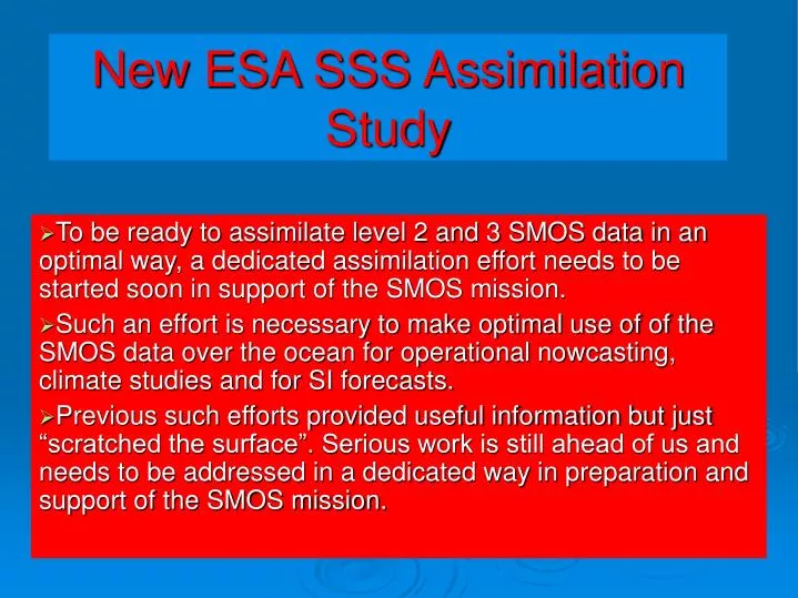
To be ready to assimilate level 2 and 3 SMOS data in an optimal way, a dedicated assimilation effort needs to be started soon in support of the SMOS mission.

E N D
To be ready to assimilate level 2 and 3 SMOS data in an optimal way, a dedicated assimilation effort needs to be started soon in support of the SMOS mission. Such an effort is necessary to make optimal use of of the SMOS data over the ocean for operational nowcasting, climate studies and for SI forecasts. Previous such efforts provided useful information but just “scratched the surface”. Serious work is still ahead of us and needs to be addressed in a dedicated way in preparation and support of the SMOS mission. New ESA SSS Assimilation Study
Goals To understand the best use of new level 2 or level 3 SSS products for operational nowcasting efforts (filtering) To understand the impact of new SSS estimates for dynamically consistent climate studies, including SI forecasting. To understand the impact of new SSS data on estimates of surface freshwater fluxes. To understand the complementarity of ARGO and SMOS data in ocean assimilation studies. All problems were not considered in previous studies but will determine the success of the data for ocean studies.
SSS observations will serve in various ways for model and state estimation studies: To provide improved information about a time-varying near surface salinity field. Presently only the Levitus monthly SSS climatology is available with large data-void areas. Time-varying anomalies from the climatology on all space and time-scales are not available in any systematic fashion. Near-surface SSS has a profound impact on the evolution of the surface mixed layer, its depth range as well as its temperature and air-sea coupling (barrier layer, pressure gradient). Improved information about the near-surface stratification has thus impact on surface heat flux estimates (at least regionally) and on atmosphere-ocean gas exchanges.
SSS observations will serve in various ways for model and state estimation studies: By constraining SSS in the estimation (assimilation) procedure (in addition to SST) it can be expected that estimated surface fluxes of heat and freshwater become much more consistent with ocean observations than feasible now. With simple assimilation approaches: Impact on sea level and the use of altimetry in ocean models. It is hoped that this route will lead to substantially improved precip. information over the ocean which otherwise is extremely difficult to measure.
Differences in Precipitation Fields Mean SSS fields from the NCAR model forced with the indicated precipitation fields, and the World Ocean Atlas (WOA98) field. Significant differences in response among the inputs are evident in all ocean basins, and with WOA98. Bill Large, NCAR (2002)
CMAP Precip. Ocean models are forced by E-P Comparison of different mean precipitation products: • large differences • large errors for SSS
Fraction of the ocean where the difference in salinity change forced by various precipitation data sets is likely to be detected. The range of ΔS among the OGCM outputs with time intervals of 1 month, 3 months, 1 year and 3 years; shown as the ratio to the Aquarius measurement error. Bill Large, NCAR, 2002
LEVITUS ORCA Model/LODYC (J.P. Boulanger, S. Masson) Mean SSS from Levitus and the two different simulations and differences Note the large differences (> 0.4 psu) at large scales => much larger than the expected SMOS noise
Rms of SSS variations from ORCA simulations (LODYC) Two reference simulations with different precipitation fields (ECMWF reanalysis and CMAP) Rms of differences = our today knowledge of SSS in the tropics. Errors range from 0.2 to 0.4 psu Scales of variability are about 4° (e.g. Lagerloef/Delcroix, 2000). A these scales, SMOS noise should be below 0.05 psu (i.e. improvement by a factor of 7) = unique contribution of SMOS given the important role (and impact) of SSS on ocean dynamics and climate in the tropics (e.g. barrier layer, buoyancy forcing, El Nino, Indian ocean dipole, impact on sea level)
December 1997 SST Anomalies Reference exp. : SST anomaly regarding to the December mean SST difference between reference exp. and perturbation exp. Min=-2,5°C Max=1,5°C Min=-0,5°C Max=0,3°C The characteristic SST anomalies of the dipole mode are reinforced by 20% when salt is involved in the vertical stratification
Previous assimilation pilot studies: Mercator/Mersea OSSE (supported by ESA) ECCO Study in support of Aquarius (unsupported)
Research Platforms Earth observing satellites Model simulations and assimilation on super computers Autonomous in situ observing systems Elements of Operational Oceanography
MERCATOR/MERSEA OSSE Overview (impact of SSS data for operational nowcasting) • Objectives • Originally: conduct experiments to assimilate three different sets of synthetic SSS level-3 products (SMOS, AQUARIUS and SMOS+AQUARIUS), and to compare their performances through so-called “Observing System Simulation Experiments”. • In practice: • Sensitivity studies to level products • Which level of SSS product is the most efficient for the new MERCATOR Assimilation System SAM2? • Sensitivity studies to observation errors • Accuracy of SMOS level-2 products? Observation errors specification ? • Sensitivity studies to observing systems • Relative skills of SMOS and AQUARIUS products? Incremental benefit of their combination?
OSSE Ingredients • REFERENCE or CONTROL RUN • Hindcast experiment with in-situ, SST and altimeter data assimilation over 2003. • OPA model: MNATL(1/3°) covering North Atlantic from 20°S to 70°N, with an eddy-permitting resolution (1/3°) • ECMWF daily forcing fluxes and a weak SST relaxation (40 W/m2) • DATA ASSIMILATION SCHEME: SAM2 • Based on a SEEK filter : Reduced Order Kalman Filter (modal space) • 3D multivariate background error covariances: 140 seasonal 3D modes (ψ,T,S) calculated from an hindcast exp. (7 years) • Innovation vector: FGAT method, observation operator for largest scales • TRUTH • The native sea surface salinity (SSS) located on the SMOS L2 data points • The native SSS comes from the North Atlantic and Mediterranean high resolution (1/15°) MERCATOR OCEAN prototype named PSY2V1 re-sampled at a 1/3° • DIAGNOSTIC • Mean and variance of misfit between OSSEs and “truth” SSS (1/3°) located on SMOS L2 data points.
Simulated SSS products computed by CLS Level (spatial and time resolution) Observation error range (RMS in PSU) SMOS L3P Level 3 SMOS (map of 200kmx200km, 10 days) 0,02 - 0,5 SMOS L2P Level 2 SMOS (40kmx40km along tracks , daily) – pixel scale 0,2 - 2,5 Aquarius L2P Level 2 Aquarius (100kmx100km along tracks, 1 daily) – pixel scale 0,1 - 1,5 Characteristics of simulated SSS data Aquarius L2 SMOS L2 SMOS L3
OSSE : main results • Conclusions from comparisons between simulations with or without simulated data : • SMOS L2 cover have a more important impact for our operational system than Aquarius L2 cover • L2 products are more suitable for our operational system than L3 products Variance of misfit SMOS L2 vs SMOS L3 Difference in variance (psu2) Aquarius L2 vs SMOS L2 Difference in variance (psu2)
AQUARIUS L2 SMOS L2 + AQUARIUS L2 0,4353 0,3077 Summary/Conclusions L2 vs L3/SMOS vs Aquarius Experiments with simulated SSS data REFERENCE or Control run SMOS L3 SMOS L2 RMS difference (PSU) between experiments and “truth” overall the domain (year 2003) 0,4859 0,3945 0,3104 The assimilation of native SMOS level-2 product is a better approach than the assimilation of gridded level-3 products, at least in the context of high-resolution models of the ocean circulation (to be expected) In the case of the assimilation of Level 3 products, it should be suitable to have a “daily Level 3 products” for our assimilation system. It should be better to assimilate SSS products with spatial resolution close to the ocean model resolution (dependent on assimilation approach). The impact of the Aquarius L2 Products is weak compared to the SMOS L2 Products: it is quite equivalent to the SMOS L3 Products (depends on data resolution). The combination of the two L2 Products has thus a small effect on final results (depends on approach). Further studies are necessary to better understand the weak impact of the Aquarius L2 Products. Combining SMOS and Aquarius Products on the same time and space scales (should be done by model)
Experiments with Simulated SSS data REFERENCE or Control run SMOS L2_2 (2 x obs. Error) SMOS L2 (native obs. Error) SMOS L2_0.5 (½ x obs. Error) RMS difference (PSU) between experiments and “truth” overall the domain (year 2003) 0,4859 0,4114 0,3104 0,2847 Discussions/Conclusions Observation errors 6. The use of SMOS L2 products give satisfactory improvement in the model, since it provides a measurable impact of the quality of ocean estimates from operational systems. 7. The observation error variance as specified by CLS (Boone et al., 2005) is a minimum requirement to extract the best possible information from SSS measurements in the context of the MERCATOR ocean forecasting system available today.
The Potential of SSS Observations for Ocean State Estimate The goal of ocean state estimation is to combine all available and diverse ocean data with a numerical model to obtain a dynamically consistent estimate of the time-evolving flow field and its uncertainties. Results can be used to study the ocean, its surface fluxes (including run-off) and its impact on climate through heat and freshwater transports and related surface fluxes.
Method: Synthesis of all available Observations to obtain dynamically consitent description of ocean circulation. Used to estimate climate change; estimate oceans uptake of CO2; initialize coupled models; now-casting of Ocean currents. GECCO Data Assimilation
Methode Cost Function Model Penalty-function type cost function The model can be imposed upon the objective function either by using Lagrange multipliers (constrained optimization), or in an unconstrained optimization form with a penalty-function type of formulation.
In the adjoint formalism a giant non-linear optimization problem is solved by iteratively changing control parameters until a statistical minimum is reached. Ongoing optimizations are run over 50 years now in one sweep. In compressed form: the forward model leads to a measure of the mode-data misfit. This misfit is input to the adjoint model (running backward in time) which in turn provides the sensitivity of the function to control parameters. Fed into a descent algorithm a new control state is determined, etc.
Consistency of Assimilation Filtered Estimate: x(t+1)=Ax(t)+Gu(t)+(t) x: model state, u: forcing etc, : data increment Data Smoothed Estimate: x(t+1)=Ax(t)+Gu(t) Data increment: time Model Physics: A, G The temporal evolution of data-assimilated estimates is physically inconsistent (e.g., budgets do not close) unless the assimilation’s data increments are explicitly ascribed to physical processes (i.e., inverted). (I. Fukumori)
Control terms usually include the initial model conditions as well as surface forcing of momentum, heat and freshwater. Thereby center provided meteorological forcing fields are adjusted to best fit ocean observations. An essential element is the existence of prior error estimates of the data, the meteorological fields and the model itself. Uncertainties of forcing fields are very poorly known. Especially precipitation over the ocean is almost entirely unmeasured and center provided estimates are having accordingly huge error bars, presumably ranging from 0.5 to 1 STD of the time varying field. Here especially much improvement is expected from SMOS data.
The Mean Ocean Circulation, global Maximenko, Niiler et al. Time-mean SSH; 1992-2003
Surface Heat Flux Estimates 100 W/m^2 -100 100 -100
Estimates of un-observables: Global Ocean Heat and Freshwater Transports o G&W o o o Interannual Variations
OGCM experiment assimilating an artificial SSS field to infer E-P forcing. In this study we performed an ocean optimization by assimilating ocean observations into an OGCM to estimate the ocean state over time and simultaneously calculates the necessary surface flux adjustments needed to match the forcing fields to the ocean state (Stammer et al., 2002).
The experiment began with the optimized state of the ocean model that had initial conditions and surface fluxes adjusted to match ocean observations. All of the conditions where then held fixed, except that the E-P temporal variability in the flux adjustments was enhanced by a factor of 4 while the mean E-P adjustment remained the same. The model was then run forward with the E-P variability enhancement and the new surface and subsurface salinity fields were computed and retrieved. These output fields constituted an artificial data set for the final step of the experiment.
In the final step, a new ocean optimization was computed treating the artificial SSS and subsurface fields as "observations" in the assimilation. The goal was to ascertain how well the artificially enhanced surface E-P flux adjustments could be reproduced. In principle, the mean adjustment should remain constant, and the variability should match the factor of four enhancement used to generate the artificial salinity.
Main results: The results were not as anticipated and are not yet fully understood. Increasing the E-P variability changes the time-mean state of SSS (through changes convection). In the optimization the main change was therefore projected on the time-mean E-M, not the “weather”. It has to be investigated if this is a general result or if – as expected – ocean state estimation can improve our estimates of surface fluxes. The experiment demonstrates the power of ocean state estimation with salinity data for constraining E-P fluxes. It is also successful in pointing out potential problems in this type of calculation that need to be understood prior to the launch of SMOS.
A more comprehensive analysis of the results needs to be carried out, but also a more comprehensive understanding of how SMOS and Aquarius data can be assimilated. The finding that E-P variability leads to changes in the mean state is scientifically very interesting as well, and may lead to new insights about how the ocean responds to an amplified water cycle as we proceed with follow-on investigations. We have to investigate to what extend the complementarity of satellite and in situ data can help reaching SMOS goals.
DeltaS = 0.1 corresponds to ~ 10cm/yr uncertainties in (E-P) - a value much lower than present 0.5 - 1 m/yr error estimates. Precipitation fields yield errors on modeled SSS of up to 0.2 to 0.4 psu to be compared to a 0.1 psu accuracy (or better depending on scales) that could be achieved with SMOS. Uncertainties for SSS should be as low as 0.01 psu. Presently variations, e.g. of the initial state are +- 0.1 psu and SSS observations with similar uncertainties would only be of marginal value for constraining S0. Even with 0.1 psu accuracy, SSS observations will have an impact on the estimation of E-P and thus P. Very positive impact of SMOS in the equatorial/tropical regions is expected. Better representation of the ocean state (currents, sea level), model improvements and possibly better seasonal forecasts. This has to be quantified with data assimilation studies.
Improving level 3 SSS data base Use the multi-mission concept Intercalibration Assimilation of SMOS/Aquarius combined products on the same time and space scales as the SMOS L2 Products. Assimilation in a global model (low and high resolution; e.g., what is the expected impact in the Pacific region?) Improving DA schemes for now casting and hind casting Control of fluxes in the assimilation scheme Combine SMOS and Aquarius with ARGO data Improve prior error description: Handling of correlated data errors and biasses. Test potential of TB assimilation. PERSPECTIVES for new ESA Study (1)
Improving DA results Use twin-experiments to test optimal assimilation strategy for operational now- hind casting and initialization of coupled models. Improving Surface Flux Estimates Use SSS in combination with other estimates of surface net E-P freshwater fluxes to improve our understanding of net precip. Over the ocean. PERSPECTIVES for new ESA Study (2)
CLIPPER SIMULATIONS - CONCLUSIONS / IMPACT ON SMOS (2) The SSS variability is larger than 0.2 psu and 0.1 psu in, respectively, 40% and 70% of the Atlantic Ocean. The SSS variability at length scales larger than 300 km (that can potentially be retrieved by SMOS) represent more than 70% of the total variability. The small scale SSS (length scales < 300 km) will add a noise to SMOS measurements generally below 0.1 psu and in some places larger than 0.5 psu. This noise will remain (much) smaller than the instrumental noise (larger than 1 psu) and will not affect much the estimation of mean (200 km x 200 km x 10 days) SSS fields from SMOS. In-situ estimations of SSS (e.g. Argo) will be much more affected by the small scale SSS. The estimations of mean fields from sparse in-situ data are thus likely to be (much) less accurate than the ones derived from SMOS (but in-situ data should allow a precise calibration of SMOS). The sampling requirements to resolve the mesoscale signals should be about 10 days and less than 100 km. This means that the effective (i.e. at these scales) noise from SMOS will be probably larger than 0.2 or 0.3 psu. Only areas of large mesoscale variability should thus benefit from SMOS observations. The large scales SSS variations are the ones that will be best observed from SMOS. Variations are typically between 0.05 and 0.5 psu rms. With a noise of 0.1 psu for 2°x2°x10d boxes, a signal of 0.1 psu at scales of 1000 km “should be observable” with a 20% error, while the error drops to below 10% for the seasonal signal (which is much better than our present knowledge of the SSS seasonal cycle) and better for the interannual signals.
SSS measurements with a 0.1/0.2 psu accuracy over 2°x2°x10 days = large improvement on our present knowledge of SSS variations Main issues for a data assimilation study Impact of SSS observations in ocean models via data assimilation • from simple methods (relaxation) to more sophisticated ones (4D-VAR, EnKF). • Effects of model biases and model errors. • Joint assimilation of in-situ and SMOS satellite data • Assimilation of averaged SSS fields at different space and time scales. Assimilation of TB or SSS. • Impact on ocean state estimation, thermohaline circulation, on seasonal forecasts for different scenarii.