Download
1 / 1
10 likes | 118 Views
LAPW: Spin polarized DFT (collinear) GGA (PBE) and LDA k=12x12x12 (hcp), k= 6x12x12 (orthorhombic) R MT K max =9.0 with R MT =2.0 3s, 3p, 3d, 4s, and 4p as valence electrons Equation of State Elasticity from strain energy density (isochoric strain)

E N D
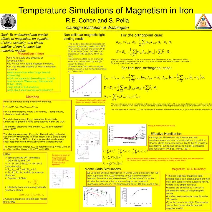
LAPW: • Spin polarized DFT (collinear) • GGA (PBE) and LDA • k=12x12x12 (hcp), k= 6x12x12 (orthorhombic) • RMTKmax=9.0 with RMT=2.0 • 3s, 3p, 3d, 4s, and 4p as valence electrons • Equation of State • Elasticity from strain energy density (isochoric strain) • Accurate magnetic tight-binding model fit to LAPW Myrasov et al. (1992) LMTO TB Sjostedt and Nordstrom (2002) LAPW Temperature Simulations of Magnetism in Iron R.E. Cohen and S. Pella Carnegie Institution of Washington Goal: To understand and predict effects of magnetism on equation of state, elasticity, and phase stability of iron for input into materials models. Non-collinear magnetic tight-binding model For the orthogonal case: • The model is based on an accurate non-magnetic tight-binding model fit to LAPW (Wasserman, Stixrude and Cohen, PRB 53, 8296, 1996; Cohen, Stixrude, and Wasserman, PRB 56, 8575, 1997; 58, 5873). • Magnetism is added via an exchange interaction parameterized by a single tensor, the Stoner I. • Problems were found with the original implementation of this method (Mukherjee and Cohen, 2001). Magnetism in iron • bcc-Fe is stable only because of ferromagnetism • fcc-Fe has no ordered magnetic moments, • but has local disordered or incommensurate moments • leads to anti-Invar effect (huge thermal expansivity) • would not appear in phase diagram if not for local moments (Wasserman, Stixrude and Cohen, 1996) • huge effect on bulk modulus • what about shear modulus and plasticity? Where h is the Hamiltonian, t is the non-magnetic part, j labels each atom, L labels each orbital, mjL is the moment from orbital L on atom j, IjLjL’ is the exchange interaction of orbital L’ on orbital L On atom j, σ is the Pauli spin tensor. For the non-orthogonal case: Methods Comparison of LAPW and TB total energies (above) and moments (below) for bcc Fe. • Multiscale method using a variety of methods. • F(V,T,,)=Fstatic+Fel+Fphonon+Fmag • For the free energy F, where V is volume, T, temperature, • structure, and strain. The static free energy Fstatic is obtained by accurate Linearized Augmented Plane computations within the GGA. The thermal electronic free energy Fstatic is also obtained using LAPW. The phonon free energy Fphonon is obtained using molecular Dynamics or the particle in a cell model with a tight-binding (TB) model fit to LAPW, or first-principles lattice dynamics linear response within the quasiharmonic approximation. The magnetic free energy Fmag is obtained using Monte Carlo on an effective Hamiltonian fit to TB and LAPW. The non-orthogonal case is complicated by the non-diagonal overlap matrix. All of our computations are non-orthogonal. Our present results use a Stoner tensor such that 3d states polarize only d states, and there is no exchange interaction for s and p. The I’s were fit to give the same magnetization energies as LAPW at each volume for bcc, and then used as a function of V for other structures. The code operates in 3 modes: (1) Find self-consistent moments and moment directions, (2) Constrain moment directions, find self-consistent moments for those directions, (3) Constrain moment magnitudes and directions. The latter 2 modes are implemented by finding staggered fields b that give the required constraints. A self-consistent penalty function method was used. It was also necessary in some cases to constrain the atomic charge so that charge does not unphysically flow during spin polarization. Energy vs moment for fm bcc Fe (left). 50 au 60 au Effective Hamiltonian 70 au 80 au Although the TB model is much faster than self-consistent electronic structure calculations, it is still too slow for Monte Carlo simulations. We fit the TB results to an effective Hamiltonian similar to that of Rosengaard and Johansson (PRB 55, 14975, 1997). 90 au Myrasov et al. (1992) LMTO TB Comparison of results for spin-wave moments (right) and energies (below) in fcc Fe. There is good qualitative agreement. Sjostedt and Nordstrom (2002) LAPW For initial tests we used only first neighbors and no K terms. The parameters Jk and Ak were determined from The TB model for FM and AFM bcc energies as functions of moment at each volume. Monte Carlo Simulations Magnetism in Fe: Summary We used the Effective Hamiltonian in Monte Carlo simulations for 128 atom supercells for 800,000 sweeps through all the degrees of freedom. The results are shown below. The “error bars” show the 1 std. dev. fluctuations in the moment—they do not represent uncertainty in the mean. The experimental Tc is 1043 K at V=79.5 au. • The non-collinear magnetic tight-binding model is in good agreement with most self-consistent calculations for Fe. • There is no empirical input. • Results are sensitive to I, which is obtained by fitting to first-principles results • An effective Hamiltonian was fit to the TB results. • Tc for bcc iron is too high. This may be due to the current simple nearest neighbor model.