Download
1 / 32
330 likes | 524 Views
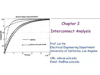
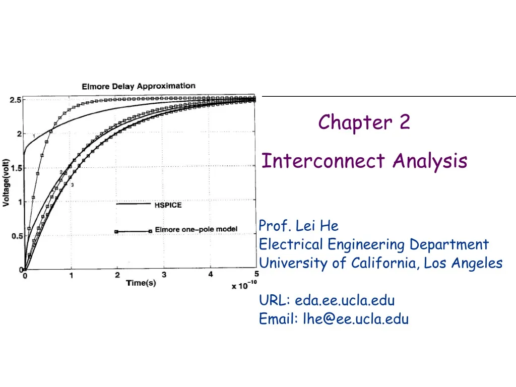
Chapter 2 Interconnect Analysis. Prof. Lei He Electrical Engineering Department University of California, Los Angeles URL: eda.ee.ucla.edu Email: lhe@ee.ucla.edu. Organization. Chapter 2a First/Second Order Analysis Chapter 2b Moment calculation and AWE General Moment Matching Models

E N D
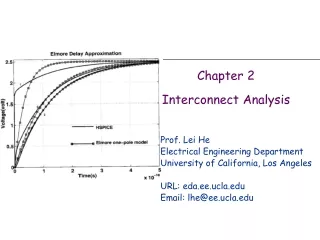
Chapter 2Interconnect Analysis Prof. Lei He Electrical Engineering Department University of California, Los Angeles URL: eda.ee.ucla.edu Email: lhe@ee.ucla.edu
Organization • Chapter 2a First/Second Order Analysis • Chapter 2b Moment calculation and AWE • General Moment Matching Models • Moments Computation • AWE • Chapter 2c Projection based model order reduction
Pade Approximation • H(s) can be modeled by Pade approximation of type (p/q): where q < p << N Or modeled by q-thPade approximation (q << N): Formulate 2q constraints by matching 2q moments to compute ki & pi
(ii) General Moment Matching Technique • Basic idea: match the moments m-(2q-r), …, m-1, m0, m1, …, mr-1 When r = 2q-1: (i) initial condition matches, i.e.
Compute Residues & Poles EQ1 match first 2q-1 moments
Basic Steps for Moment Matching Step 1: Compute 2q moments m-1, m0, m1, …, m(2q-2) of H(s) Step 2: Solve 2q non-linear equations of EQ1 to get Step 3:Get approximate waveform Step 4:Increase q and repeat 1-4, if necessary, for better accuracy
Components of Moment Matching Methods • Moment matching methods • 2-pole method (S2P introduced previously) • Asymptotic Waveform Evaluation (AWE) [Pillage-Rohrer, TCAD’90] • Critical Component • Moment computation
Organization • General Moment Matching Models • Moments Computation • AWE
Basis of Moment Computation by DC Analysis • Applicable to general RLC networks • Used in Asymptotic Waveform Evaluation (AWE) • Represent a lumped, linear, time-invariant circuit by a system of first-order differential equations: • where xrepresents circuit variables (currents and voltages) • G represents memoryless elements (resistors) • C represents memory elements (capacitors and inductors) • bu represents excitations from independent sources • y is the output of interest
Transfer Function • Assume zero initial conditions and perform Laplace • transform: • where X, U, Y denote Laplace transform of x, u, y, respectively Transfer function: Let s = s0 + s, where s0 is an arbitrary, but fixed expansion point such that G+s0C is non-singular
Taylor Expansion and Moments • Expansion of H(s) about s= 0: Recursive moment computation:
Taylor Expansion and Moments (Cont’d) • Expansion of H(s) around Recursive moment computation:
When s0 = 0, equivalent to DC analysis: • setting shorting inductors (0V) and opening capacitors (0A) • compute currents through inductors and voltages across capacitors as moments Inductor Voltage source Capacitor Current source Interpretation of Moment Computation • Compute: • Convert:
When s0 = 0, equivalent to DC analysis: • setting voltage sources of inductor L= LmL, current sources of capacitor C = CmC • external excitations = 0 • compute currents through inductors and voltages across capacitors as moments Inductor Voltage source Capacitor Current source Interpretation of Moment Computation (Cont’d) • Compute: • Convert:
When s0 = 0, equivalent to DC analysis: • setting moments as currents through inductors and voltages across capacitors • external excitations = 0 • compute voltage sources of inductors and current sources of capacitors Inductor Voltage source Capacitor Current source Interpretation of Moment Computation (Cont’d) • Compute: • Convert:
Moment Computation by DC Analysis • Perform DC analysis to compute the (i+1)-th order moments • voltage across Cj => the (i+1)-th order moment of Cj • current across Lj => the (i+1)-th order moment of Lj • DC analysis: • modified nodal analysis (used in original AWE ) • sparse-tableau • …… • Time complexity to compute moments up to the p-th order: p time complexity of DC analysis
Advantage and Disadvantage ofMoment Computation by DC Analysis • Recursive computation of vectors uk is efficient since the matrix (G+s0C) is LU-factored exactly once • Computation of uk corresponds to vector iteration with matrix A • Converges to an eigenvector corresponding to an eigenvalue of A with largest absolute value
Organization • General Moment Matching Models • Moments Computation • AWE
Moment Matching by AWE[Pillage-Rohrer, TCAD’90] • Recall the transfer function obtained from a linear • circuit • Let s = s0 + s, where s0 is an arbitrary, but fixed expansion point such that G+s0C is non-singular • When matrix A is diagonalizable
q-th Pade Approximation • Pade approximation of type (p/q): q-thPade approximation (q << N): Equivalent to finding a reduced-order matrix AR such that eigenvalueslj of AR are reciprocals of the approximating poles pj for the original system
Asymptotic Waveform Evaluation • Recall EQ1: • Let
Asymptotic Waveform Evaluation (Cont’d) • Rewrite EQ1: where Solving for k: Let Need to compute all the poles first
Structure of Matrix AR • Matrix: has characteristic equation: • Therefore, AR could be a matrix of the above structure • Note that: Characteristic equation becomes the denominator of Hq(s):
Solving for Matrix AR • Consider multiplications of ARon ml produces produces
Solving for Matrix AR (Cont’d) • After q multiplications of ARon ml produces Equating m’ with m:
Summary of AWE Step 1: Compute 2q moments, choice of q depends on accuracy requirement; in practice, q 5 is frequently used Step 2: Solve a system of linear equations by Gaussian elimination to get aj Step 3:Solve the characteristic equation of AR to determine the approximate poles pj Step 4:Solve for residues kj
Numerical Limitations of AWE • Due to recursive computation of moments • Converges to an eigenvector corresponding to an eigenvalue of matrix A with largest absolute value • Moment matrix used in AWE becomes rapidly ill-conditioned • Increasing number of poles does not improve accuracy • Unable to estimate the accuracy of the approximating model • Remedial techniques are sometimes heuristic, hard to apply automatically, and may be computationally expensive
[1] Given the circuit as shown below and a unit step voltage source at the input node s, use SPICE to simulate the circuit and obtain the accurate 50% delay at node n. Also analytically calculate the delay using Elmore method and S2P method. How do they compare with the result obtained by SPICE? Homework R4 R2 C4 C2 R1 s R3 R5 C5 C1 n 1v C3 R1 = 1mΩ R2 = 2mΩ R3 = 2mΩ R4 = 1mΩ R5 = 4mΩ C1 = 1nF C2 = 1nF C3 = 4nF C4 = 4nF C5 = 2nF
R4 R2 C4 C2 R1 s R3 C6 C5 C1 n 1v C3 Homework [2] Give the circuit as shown below and a unit step voltage source at node s, can we still use the “shared-path” formula to calculate the Elmore delay? Explain why or why not. Use DC analysis method via MATLAB or SPICE to get the 0th -3rd moments of C3 and C5. R1 = 1mΩ R2 = 2mΩ R3 = 2mΩ R4 = 1mΩ C1 = 1nF C2 = 1nF C3 = 4nF C4 = 4nF C5 = 2nF C6 = 1nF
Steps for Problem 1 1. Write the SPICE netlist of the circuit and probe the voltage response at node n. 2. Record the time when the voltage at node n reaches 0.5V. That time is the 50% delay. 3. Use the Elmore delay formula to calculate the Elmore delay. (find the shared path between each node and node n). 4. Write down the transfer function and driving point admittance of the circuit with input s and output n. 5. Expand the transfer function to get the moments m1* and m2*. Expand the driving point admittance to get m1, m2, m3, and m4.
Steps for Problem 1 6. Follow the S2P algorithm to get k1, k2, p1 and p2. 7. Use the frequency domain expression (h(s)) to derive the time domain expression (h(t)). 8. Plot the obtained time domain waveform to get the 50% delay for the S2P model. 9. Compare the results.
Steps for Problem 2 1. Follow the DC analysis method to reconstruct the circuit (e.g. replace C with zero current source for 0th moment calculation, etc). 2. Stamp the G and C matrices for MATLAB analysis or write the corresponding netlist for SPICE analysis. 3. Get the voltage across the capacitance as the moment. 4. The above should be done repeatedly until all the desired moments are acquired.