Download
1 / 57
620 likes | 1.06k Views
Ifgi, Muenster, Fall School 2005 . Spatial Data Analysis Areas II – Exploratory Spatial Data Analysis. Gilberto Câmara INPE, Brazil. Data-Driven Approaches. “Exploratory spatial data analysis" (ESDA) Point pattern analysis Indices of spatial association

E N D
Ifgi, Muenster, Fall School 2005 Spatial Data AnalysisAreas II – Exploratory Spatial Data Analysis Gilberto Câmara INPE, Brazil
Data-Driven Approaches • “Exploratory spatial data analysis" (ESDA) • Point pattern analysis • Indices of spatial association • Compare the observed pattern in the data (e.g., locations in point pattern analysis, values at locations in spatial autocorrelation) to one in which space is irrelevant. • The second common aspect is that the spatial pattern, spatial structure, or form for the spatial dependence are derived from the data only.
Spatial Autocorrelation • Complicated name, simple concept... • Expresses the amount of spatial dependence • How much proximity matters in spatial data • Correlation is the key notion • It indicates how much two properties vary together • Correlation in space • Is a variable in a location correlated with its values in nearby places? • Spatial + auto + correlation
Sometimes we need to transform the data Scatter plots: (a) Y versus PORC3_NR (percentage of large farms in number ); (b) log10 Y versus log 10 (PORC3_NR). Predicted versus Observed Plots: (a) model with variables not transformed): R2 = 0.61; (b) Model 7: R2 = 0.85.
Log x linear correlation • Y = aX - linear corellation • Y = Xa or log Y = a logX – log correlation
6 4 2 Y 0 0 20 40 60 -2 -4 -6 X No Correlation
Spatial Randomness • Null Hypothesis: No Spatial Autocorrelation • Spatial randomness • values observed at a location do not depend on values observed at neighboring locations • observed spatial pattern of values is equally likely as any other spatial pattern • the location of values may be altered without affecting the information content of the data
Random or Clustered? Columbus homicide data (source: Luc Anselin)
Random or Clustered? Columbus homicide data (source: Luc Anselin)
Random or Clustered? Columbus homicide data (source: Luc Anselin)
Exploratory Spatial Data Analysis • Visualization of spatial data • Global Indicators of Spatial Autocorrelation • Local Indicators of Spatial Autocorrelation (LISA)
Visualization of Area Patterns • Grouping • Equal intervals • Quantiles • Standard deviation • Be careful! • Color mapas can lead to wrong interpretation Breast cancer in England (1985-1989) Source: Bailey and Gattrel, 1995
Equal-Interval Visualization • Defined by maximum and minimum values. • Shows data dispersion. • “Outliers” can mask differences. Source: Bailey and Gattrel, 1995
Quantiles • Each group has the same numbre of elements • Ordenation • e.g: best 25% and worst 25% Source: Bailey and Gattrel, 1995
Standard Deviations • Dispersion around a mean value • Breaks: 1 stdev, 1/2 stdev • Shows the statistical behaviour • Best for normality case Source: Bailey and Gattrel, 1995
Visualization Source: Bailey and Gattrel, 1995
Visualization Source: Bailey and Gattrel, 1995
C B A E D A B C D E A 0 1 0 1 0 B 1 0 1 1 1 C 0 1 0 0 1 D 1 1 0 0 1 E 0 1 1 1 0 Spatial Proximity Matrix • Matrix W (n x n) , where each elements wij represents a measure of nearness between Oiand Oj • Criteria: wij =1, if Oi touches Oj wij= 1,if distance(Oi,Oj) < h
Moving Averages • Local smoothing of attribute values where: • Wij is the spatial weights matrix. • yi is the attribute value for each area. • n is the number of areas
Standard Deviations Moving Averages Moving Averages Proportion of population aged 70 or older, São Paulo, 1991
Moving Averages using Bar Graphs Regions where there is a large difference between the original value and the local mean Indicates places of spatial transitions Atributo Média local
Moran Scatterplot: Values x Local Means Q1 (val. [+], means [+]) and Q2 (val. [-], means [-]) Locations of positive spatial association (“I’m similar to my neighbours”). WZ Q4 Q1 a 0 Q3 (val. [+], means [-]) and Q4 (val. [-], means [+]) Locations of negative spatial association (“I’m different from my neighbours”). Q2 Q3 z 0
Moran Scatterplot Map São Paulo WZ Q4 = LH Q1= HH a 0 Q2= LL Q3 = HL z 0 Old-aged population
n n n å å å G = G = w a w a i ij ij ij ij i j j w ij Indicators of spatial autocorrelations • Generic formulation: global local where : spatial proximity between i and j a : measured relation between object and its neighbors ij
Indicators of spatial autocorrelation n n n å å å G = G = w a w a i ij ij ij ij i j j ( ) ( ) Moran (covariance) z z - - x x x x i j i j ( ) ( ) 2 2 Geary (variance) - - z z x x i j i j ( ) ( ) + x ou x x G or G* (moving averages) + z ou z z j i j j i j
Global Indicators of Spatial Autocorrelation • Moran’s I: onde: • n number of areas, • yi attribute value in area i, • mean value in study region • wij spatial weigths matrix. • How to interpret the above equation?
Global Indicators of Spatial Autocorrelation • Similar to tradicional correlation calculation, but restricted to spatial neighbours • Values of I go from -1 to +1. • -1 negative spatial autocorrelation • 0 no spatial autocorrelation • +1 positive spatial autocorrelation • For the old-age population in São Paulo, I=0.45 • Is this significant?
Randomization Strategy • Empirical Distribution Function • permute arrangement of objects • associate values with locations • associate locations with values • recompute indicators • Obtain a distribution • Compare observed Γ to distribution of pseudo-Significance • p = (t + 1) / (m + 1) • M: # permutations; • T: # times ΓAW ≥ Γ
Random or Clustered? • Testing Moran’s I • Permutate the spatial values 999 times • Obtain a probability distribution • Locate the “real” value in the distribution • In this case, I = .45 (very significant!) extremo Distribuição simulada
Pros and cons of randomization • Advantages • non-parametric • no distributional assumptions • easy to compute • easy to interpret • Disadvantages • sample specific • no generalization to population • precision of pseudo significance arbitrary • 1/(99+1) yields 0.01, and 1/(999+1) yields 0.00 • sensitive to random number generator
Random or Clustered? Moran’s I = -0.003 Moran’s I = 0.486 Columbus homicide data (source: Luc Anselin)
Spatial Analysis What distinguishes spatial statistical data analysis is that its main focus is on inquiring about spatial patterns of places and values, the spatial association between them and the sistematic variation of the phenomenon in diffeent locations. Anselin,1992
Local Indicators of Spatial Autocorrelation (LISA) • Moran’ I is global • What if we want to find out the spatial correlation of each area? • Use a local indicator • Compares local value to that of its neighbours
Local and Global Analysis • Global • one statistic to summarize pattern • Clustering • Homogeneity • Local • location-specific statistics • clusters • heterogeneity
LISA Definition (Anselin 1995) • LISA satisfies two requirements • indicate significant spatial clustering for each location • sum of LISA proportional to a global indicator of spatial association • LISA Forms of Global Statistics • local Moran, local Geary, local Gamma
Use of LISA • Identify Hot Spots • significant local clusters in the absence of global autocorrelation • some complications in the presence of global autocorrelation (extra heterogeneity) • significant local outliers • high surrounded by low and vice versa • Indicate Local Instability • local deviations from global pattern of spatial autocorrelation
Local Indicators of Spatial Autocorrelation (LISA) LISAs enable a quantitative expression of spatial distribution of values Distributution characteristics -concentrations -persistences -transitions
Local Indicators of Spatial Autocorrelation (LISA) Local Moran G index where is the spatial weight for objects i and j
Distance Statistics for Local Spatial Association • Getis-Ord Gi and Gi* • one statistic for each location • contiguity as distance bands, wij(d) • Gi Statistic • does not include observation i • Gi* Statistic • includes observation i in sum
Interpretation of Gi Statistics • Local Spatial Association • positive: clusters of high values • negative: clusters of low values • Inference • randomization • permutation • Visualization • map of locations with significant Gi or Gi*
Local Indicators of Spatial Autocorrelation (LISA) • How can we know if a LISA value means anything? • Use permutation to construct a probability distribtuion • Change everybody’s place but one region • Produce a map showing those areas whose LISA values are different from the rest (“LISA MAP”). • Statistical Significance • Not significant • Significant at 95% (1,96s), 99% (2,54s) e 99,9% (3,2s).
% old-age Not significant p = 0.05 [95% (1,96s)] p = 0.01 [99% (2,54s)] p = 0.001 [99,9% (3,2s)] LISA Map for old age in São Paulo
proportion of jobs per local population in greater São Paulo Data
ANÁLISE ESPACIAL II - LISA Mapa Gi* normalizado classificados por desvios padrão
Guarulhos São Miguel Osasco Sto. André S. Bernardo ANÁLISE ESPACIAL II - LISA Mapa de Espalhamento de Moran
Interpretation and Limitations • Most Important • assessing lack of spatial randomness • suggests “significant” spatial structure • Multivariate Association • univariate spatial autocorrelation may result from • multivariate association • scale mismatch • need to control for other variables = spatial regression • LISA Clusters and Hot Spots • suggest interesting locations • do not explain