Download
1 / 13
140 likes | 251 Views
Department of Meteorology & Climatology FMFI UK Bratislava. Davies Coupling in a Shallow-Water Model. Mat úš M ART ÍNI. Arakawa , A., 1984. Boundary conditions in limited-area model. Dep. of Atmospheric Sciences. University of California, Los Angeles: 28pp.

E N D
Department of Meteorology & Climatology FMFI UK Bratislava Davies Couplingin a Shallow-Water Model Matúš MARTÍNI
Arakawa, A., 1984. Boundary conditions in limited-area model. Dep. of Atmospheric Sciences. University of California, Los Angeles: 28pp. • Davies, H.C., 1976. A lateral boundary formulation for multi-level prediction models. Q. J. Roy. Met. Soc., Vol. 102, 405-418. • McDonald, A., 1997. Lateral boundary conditions for operational regional forecast models; a review. Irish Meteorogical Service, Dublin: 25 pp. • Mesinger, F., Arakawa A., 1976. Numerical Methods Used in Atmospherical Models. Vol. 1, WMO/ICSU Joint Organizing Committee, GARP Publication Series No. 17, 53-54. • Phillips, N. A., 1990. Dispersion processes in large-scale weather prediction. WMO - No. 700, Sixth IMO Lecture: 1-23. • Termonia, P., 2002. The specific LAM coupling problem seen as a filter. Kransjka Gora: 25 pp.
Motivation High resolution NWP techniques: • global model with variable resolution ARPEGE 22 – 270 km • low resolution driving model with nested high resolution LAM DWD/GME DWD/LM 60 km 7 km • combination of both methods ARPEGE ALADIN/LACE ALADIN/SLOK 25 km 12 km 7 km
WHY NESTED MODELSIMPROVE WEATHER - FORECAST • the surface is more accurately characterized (orography, roughness, type of soil, vegetation, albedo …) • more realistic parametrizations might be used, eventually some of the physical processes can be fully resolved in LAM • own assimilation system better initial conditions (early phases of integration)
Shallow-water equations • 1D system (Coriolis acceleration not considered) • linearization around resting background • forward-backward scheme • centered finite differences DISCRETIZATION
Davies relaxation scheme continuous formulation inshallow-water system discrete formulation - general formalism:
PROPERTIES OF DAVIES RELAXATION SCHEME Input of the wave from the driving model u j
Difference betweennumerical and analytical solution 8-point relaxation zone (no relaxation)
Outcome of the wave, which is not represented in driving model
8-point relaxation zone analytical solution 8 72 8 72 8 8 72 8 72
Minimalization of the reflection • weight function • width of the relaxation zone • the velocity of the wave (4 different velocities satisfying CFL stability criterion) (simulation of dispersive system) • wave-length
Choosing the weight function testing criterion - critical reflection coefficient r r [%] r [%] linear convex-concave (ALADIN) cosine tan hyperbolic quartic quadratic number of points in relaxation zone
(more accurate representation of surface) DM LAM DM LAM LAM DM 8 32 8 32 8 32 DM-driving modelLAM-limited area model