Download

1 / 54
600 likes | 3.57k Views
Fundamentals of Rietveld Refinement I. XRD Pattern Simulation. An Introduction to Rietveld Refinement using PANalytical X’Pert HighScore Plus v3.0d Scott A Speakman, Ph.D. MIT Center for Materials Science and Engineering speakman@mit.edu. Outline.

E N D
Fundamentals of Rietveld RefinementI. XRD Pattern Simulation An Introduction to Rietveld Refinement using PANalyticalX’PertHighScore Plus v3.0d Scott A Speakman, Ph.D. MIT Center for Materials Science and Engineering speakman@mit.edu
Outline • Calculating a Diffraction Pattern from a Crystal Structure • Using HighScore Plus to Simulate a Diffraction Pattern • Manually Refining a Model to Match Experimental Data
The position and intensity of peaks in a diffraction pattern are determined by the crystal structure • These three phases of SiO2 are chemically identical. • Differences in the atomic structure are reflected in the diffraction patterns.
The diffraction peak position is a product of the atomic bond distances in the crystal Bragg’s Law: λ= 2dhklsinθ • Bragg’s law calculates the angle where constructive interference from X-rays scattered by parallel planes of atoms will produce a diffraction peak. • In most diffractometers, the X-ray wavelength l is fixed. • Consequently, a family of planes produces a diffraction peak only at a specific angle 2q. • The lattice parameters of the unit cell are used to calculate dhkl
dhkl is a function of the size and shape of the unit cell • dhklis the vector drawn from the origin of the unit cell to intersect the crystallographic plane (hkl) at a 90° angle. • dhkl, the vector magnitude, is the distance between parallel planes of atoms in the family (hkl) • the diffraction peak position is a product of the average atomic distances in the crystal • anything that changes the average bond distances (temperature, pressure, etc.) will change dhkl and therefore the diffraction peak positions d110
The amplitude of light scattered by a crystal is determined by the arrangement of atoms in the diffracting planes • The structure factor quantifies the amplitude of light scattered by a crystal • The patterns of atoms in the unit cell scatters strongly in some directions and weakly in others owing to interference of the wavelets scattered by the atoms • Fhkl sums the result of scattering from all of the atoms in the unit cell to form a diffraction peak from the (hkl) planes of atoms • The amplitude of scattered light is determined by: • where the atoms are on the atomic planes • this is expressed by the fractional coordinates xjyjzj • what atoms are on the atomic planes • the scattering factor fj quantifies the relative efficiency of scattering at any angle by the group of electrons in each atom • Nj is the fraction of every equivalent position that is occupied by atom j
The scattering factor, f, quantifies the efficiency of scattering from a group of electrons in an atom • X-rays are electromagnetic radiation that interact with an electron, which reradiates the X-ray as a spherical wave • The number of electrons around an atom defines how strongly it will scatter the incident X-ray beam • the initial strength of the atomic scattering factor is equal to the number of electrons around the atom • The scattering factor, f, is a product of several terms describing the interaction of the X-ray with the electrons around an atom
The atomic scattering factor f0 can be found using tables or equations determined experimentally or from quantum mechanical approximations • f0 at 0° is equal to the number of electrons around the atom • Y and Zr are similar, but slightly different, at 0° • Zr and Zr4+ are slightly different at 0° • Y3+ and Zr4+ are identical at 0° • the variation with (sin θ)/λ depends on size of atom • smaller atoms drop off quicker • at higher angles, the difference between Y3+ and Zr4+ is more readily discerned • at higher angles, the difference between different oxidation states (egZr and Zr4+) is less prominent
Thermal motion of the atom changes the scattering factor • the efficiency of scattering by an atom is reduced because the atom and its electrons are not stationary • the atom is vibrating about its equilibrium lattice site • the amount of vibration is quantified by the Debye-Waller temperature factor: B=8π2U2 • U2 is the mean-square amplitude of the vibration • this is for isotropic vibration: sometimes B is broken down into six Bij anistropic terms if the amplitude of vibration is not the same in all directions. • aka temperature factor, displacement factor, thermal displacement parameter
Anomalous scattering of X-rays with energies near the absorption edge of the atom changes the scattering factor • scattering factor has a real and imaginary term • these terms only matter when the energy of the incident X-ray approaches the ionization energy of atom • when the wavelength of the incident X-ray is near the absorption edge of the atom • anomalous scattering describes how some photons with energy approaching the ionization energy will be scattered out of phase with the majority of photons
With a crystal structure to solve Bragg’s Law and Fhkl, you can calculate the diffraction pattern from an ideal crystal • Ideal powder diffraction patterns can be simulated if you know ... • space group symmetry • unit cell dimensions • atom types • relative coordinates of atoms in unit cell • atomic site occupancies • atomic thermal displacement parameters • ... for each and every phase in the sample
Where to Get Crystal Structures • publications • Commercial Databases • Inorganic Crystal Structure Database (ICSD) • Linus Pauling File (LPF) • this is included in ICDD PDF4+ Inorganic • NIST Structural Database (metals, alloys, intermetallics) • Cambridge Structure Database (CSD) (organic materials) • Free Online Databases • ICSD- 4% available as demo at http://icsd.ill.eu/icsd/index.html • Crystallography Open Database http://www.crystallography.net/ • Mincryst http://database.iem.ac.ru/mincryst/index.php • American Mineralogist http://www.minsocam.org/MSA/Crystal_Database.html • WebMineral http://www.webmineral.com/ • Protein Data Bank http://www.rcsb.org/pdb/home/home.do • Nucleic Acid Database http://ndbserver.rutgers.edu/ • Database of Zeolite Structures http://www.iza-structure.org/databases/
A Crystal Structure • ZrO2 • Space Group Fm-3m (225) • Lattice Parameter a=5.11 site occupancy factor, sof, is equivalent to N in the Fhkl equation
Wyckoff Site notation is a shortcut to indicate if the type of site that the atoms occupies in the crystal • each letter in the Wyckoff notation specifies a site that sits on a different combination of symmetry elements • the number in the Wyckoff notation indicates the number of atoms put into the unit cell if the atom is on that site • 4a- an atom on the a site will populate the unit cell with 4 atoms • 8c- an atom on the c site will populate the unit cell with 8 atoms • Wyckoff notation gives you a quick way to check if stoichiometry is correctly preserved when you create a crystal structure • you can deduce z, the number of molecules per unit cell, from the Wyckoff notation (z=4 for ZrO2) • The Wyckoff site indicates if x, y or z are can change or if they must be fixed to preserve the symmetry of the crystal
The Site Occupancy Factor, sof, indicates what fraction of a site is occupied by a specific atom • The sof is N in the structure factor equation • sof = 1, every equivalent position for xyz is occupied by that atom • sof < 1, some of the sites are vacant • two atoms occupying the same site will each have a fractional sof • remember that the observed XRD pattern is an average of hundreds or thousands of unit cells that make a crystallite
For pattern calculations and Rietveld refinement in HSP, the “Structures” desktop is recommended • Desktops can be changed in the menu: • View > Desktops • All slides in this tutorial were created with HSP in the “Structures” desktop
With this crystal structure information, we can build a crystal in HSP • Start X’Pert HighScore Plus • Create a New Document File>New • Analysis>Rietveld>Enter New Structure
Step 1: Enter Title • Follow the entry form from top to bottom, via the numbered steps
Step 2: Enter Space Group • Each space group has a unique number (1 thru 230) • you can just enter number into the space group field • HSP will assume the standard origin and setting • You can use the drop-down menu to select a space group • You can open the symmetry explorer by clicking on the ... button
The symmetry explorer allows you to choose the space group and a specific origin, and to see information about the symmetry elements and special positions
Step 3: Enter Unit Cell • lattice parameters are automatically constrained by the space group that you chose • a cubic space group: a=b=c, a=b=g=90
Step 4: Enter Atoms • The element can be an atom or ion (select oxidation state) • the use of oxidation states in modifying the scattering factor for an atom is set in Customize>Program Settings, in the Rietveld tab • by default it is set to “Ignore Oxidation States” • name is the element by default, but it can be changed (useful if you have the same element on multiple sites) • entering Wyckoff site can save you from having to type in xyz • if you enter xyz, the Wyckoff site is automatically assigned • When finished, click OK to create that crystal structure!
We can now simulate the ideal X-Ray powder diffraction pattern in HSP • We have entered in all of the information necessary to simulate an X-ray diffraction pattern • Click on the ‘Start Pattern Simulation’ button to produce the theoretical diffraction pattern
The pattern simulation parameters can be changed in Program Settings • To change settings go to Customize> Program Settings • In Simulation tab, you can change the parameters for the simulated scan • Default range for simulation is 5 to 70 °2theta • change start and end angles to 25 and 90 °2theta • click OK to enter change and close window • click ‘Start Pattern Simulation’ again
The wavelength of radiation used in the simulation can be changed in Document Settings • To change settings go to Customize> Document Settings • In Document Wavelength tab, you can change the X-ray source used • there is an “Other” option if you used a non-characteristic wavelength, such as at a synchrotron • click ‘Start Pattern Simulation’ again
Parameters for the crystal structure and the simulation can be accessed in the Refinement Control list • the parameters for the pattern simulation are shown in the Refinement Control List • The values for global parameters and each individual crystal structure entered into the simulation are listed in a nested tree format • You can trim the number of tabs in the Lists Pane in the View menu
The Object Inspector shows additional details for any element you select in other windows • If you click on the phase name (eg Zirconia) in Refinement Control list, you will be able to see additional information about that phase in the Object Inspector • This includes information such as calculated density, chemical formula, and formula mass • You can use these to check that you created the crystal structure correctly • You can change details such as the phase name and color of simulated diffraction pattern
We want to keep this pattern as a reference during the next exercises • Go to Scan List in the Lists Pane • Right Click on the current scan that is shown in the list (which is the simulated pattern) • Select “Convert calc. Profile to obs. Profile” • Now the original simulation will remain in the Main Graphics View and we can compare it to new simulations
We can change parameters for the crystal structure and observe how they change the diffraction pattern • The unit cell lattice parameters determine where the diffraction peaks are observed • the peak intensity is determined by • what atoms are in the crystal and their positions xyz • the site occupancy of the atom • the relative scattering strength of the atom, scattering factor, which is a product of the number of electrons around the atom • the thermal parameter of the atom • This is not just useful for these tutorial purposes, but also for anticipating what your real data might look like and for evaluating limits of detection
To change values for the simulation • In the Refinement Control, • expand the Zirconia entry • Expand the Unit Cell entry • Change the Unit Cell value • After typing, you must press ‘Enter’ key to register the change • if you try recalculating the simulation without pressing enter, you may lose the changed value • recalculate the diffraction pattern by clicking on “Start Pattern Simulation” button again • change the lattice parameter and recalculate the pattern several times to get a feel for the relationship
To change atom parameters • click on Atomic Coordinates in the Refinement Control List • The atomic information appears in the Object Inspector • Expand the Object Inspector window so that you can see more clearly • You know that you are working with the atoms because the Object Inspector pane says “Selected Object: Atomic Coordinates”
Change the Site Occupancies (sof) for the atoms • Changing the occupancy of Zr has a big effect • change the SOF of Zr to 0.5 and recalculate the pattern • Changing the occupancy of O has a small effect • reset the SOF of Zr to 1.0 and change the SOF of O to 0.5, then recalculate the pattern • Remember, the atomic scattering factor, f0, is equal to the number of electrons around the atom • Zr atoms scatter much more strongly than O, so the XRD diffraction pattern is more sensitive to the Zr atoms
We can predict the change in peak intensities when we dope the sample • replace 20% Zr with Y • right click on the Object Inspector and select “add new atom” • To create the new atom, type “Y” for the Element • tab over to Wyckoff Site and type “4a” and enter • this automatically places the atom at 0,0,0 • make the sof 0.2 • make the Biso 1.14 • make the sof for the Zr atom 0.8 • This means that the 4a site is occupied by 80% Zr and 20%Y • recalculate the simulation • little change in intensity • replace 20% Zr with Ce • change the atom type of Y to Ce and recalculate the simulation • how could we quantify amount of Y doping in YSZ?
The thermal parameter, Biso, changes how scattering efficiency changes with as a function of (sin q)/l • change thermal parameter for Zr • reset the SOF of Zr to 1 and the SOF of the other 4a atom (Ce or Y) to 0 • the diffraction pattern will be representative of ZrO2 with no doping • change Biso and recalculate the diffraction pattern • change from 1.14 to 2.3 • change to 5 • change to 0.1
These simulations do not necessarily represent the data that your diffractometer will produce • There are more factors that contribute to the diffraction pattern that you collect with an instrument • Some of these factors are calculated from fundamental equations • The simulations that we have been executing already account for multiplicity, for Ka2 radiation, and for the Lorentz polarization factor • Some of these factors are approximated using empirical formulas • The simulations that we have been executing already account for the peak width due to divergence, mosaicity, resolution of the diffractometer
Other Things that effect intensity IK=SMKLK|FK|2PKAKEK • S is an arbitrary scale factor • used to adjust the relative contribution of individual phases to the overall diffraction pattern • M is the multiplicity of the reflection • accounts for the fact that some observed diffraction peaks are acutally the product of multiple equivalent planes diffracting at the same position 2theta (for example, (001) (100) (010) etc in cubic) • automatically calculated based on the crystal structure • L is the Lorentz polarization factor • P is the modification of intensity due to preferred orientation • A is absorption correction • E is extinction correction • F is structure factor, which is the amplitude of scattered light due to the crystal structure (already discussed)
The Lorentz polarization factor corrects for several effects • The Lorentz factor • Different planes remain in the diffracting condition over a different angular range • high angle planes remain in the diffracting position longer, increasing their apparent intensity • 1/sin2qcosq relationship for Bragg-Brentano • varies with geometry of the diffractometer • Polarization • Scattering of light by the atom polarizes the X-rays • this causes the scattered intensity to vary as 1+cos2(2q)/2 • Monochromator Polarization • The monochromator uses diffraction from a crystal to remove unwanted wavelengths of radiation. • This diffraction will also polarize the X-ray beam, causing intensity to vary as cos2(2q) • POL is the correction factor for the monochromator • the correct POL value can be found in HSP Help • go to the Help Index, type in POL, and the first option describes the Lorentz polarization factor
Setting the Polarization Correction Coefficient, POL, for your simulation • in the Refinement Control list, click on Global Parameters • The Global Parameters will show up in the Object Inspector • In the “General Properties” expansion of the Object Inspector, you can set the Polarization Correction Coefficient (POL)
Modeling Preferred Orientation • The default calculation assumes that there are an equal number of crystallites contributing to every diffraction peak • the orientation of the crystallites is random and there are a statistically relevant number of grains • preferred crystallographic orientation produces a non-random distribution in the orientation of the crystallites • the observed diffraction peak intensities will vary systematically
The March distribution function empirically models the preferred orientation effect • The March distribution function is a model for fitting preferred orientation of cylinder or needle shaped crystals. k is the angle between the preferred orientation vector and the normal to the planes generating the diffracted peak r is a refinable parameter in the Rietveld method we will explore using the correction in our refinement on Tuesday
Modeling Preferred Orientation in HSP • In the Refinement Control list, click on the phase that has preferred orientation • In the Object Inspector, expand the Preferred Orientation settings • set the h,k, and l directions to represent the [hkl] of the preferred orientation • set the PreferredOrientationparameter • this parameter is found in the Object Inspector as “Parameter (March/Dollase)” • this parameter is also found in the Refinement Control List as “Preferred Orientation” • 1 means the orientation of [hkl] is completely random • <1 means that the [hkl] direction is the preferred orientation of the crystallites • >1 means that the [hkl] direction is preferentially avoided • recalculate the simulation to observe the change in peak intensities
Additional Intensity Factors • Absorption Correction • accounts for the transmission and absorption of the X-rays through the irradiated volume of the sample. • depends on sample geometry: flat plate or cylindrical • depends on the mass absorption coefficient of the sample • significant for cylindrical or transmission samples with a high sample absorption • significant for a flat plate sample with a low sample absorption • Extinction Correction • Secondary diffraction of scattered X-rays in a large perfect crystal can decrease the observed intensity of the most intense peaks • scattering by uppermost grains limits the penetration depth of a majority of X-rays, causing a smaller irradiated volume • want “ideally imperfect” crystals– grains with enough mosaicity to limit extinction • better to reduce extinction by grinding the powder to a finer size • These two corrections are rarely used. Caution is advised. Always check to make sure that the correction values are physically meaningful.
We now know how to calculate the diffraction peak intensity, but there a couple of more factors involved in simulating real diffraction data • The intensity, Yic, of each individual data point i is calculated using the equation: • We already know how to calculate IK, the intensity of the Bragg diffraction peak k: IK=SMKLK|FK|2PKAKEK • Yib is the intensity of the background at point i in the pattern • k1 - k2 are the reflections contributing to data point i in the pattern • sometimes multiple Bragg diffraction peaks overlap, resulting in multiple contributions to the observed intensity at a single data point • Gik is the peak profile function • this describes how the intensity of the diffraction peak is distributed over a range of 2theta rather than at a single point • this profile is due to instrument broadening, sample broadening, etc
Sample attributes also contribute to the diffraction peak shape and width mass absorption coefficient (sample transparency) sample thickness crystallite size microstrain defect concentration Diffraction peaks have profiles that must be empirically modeled • The intensity equation Ik predicts that diffraction peak intensity occurs at a single point 2theta– but in reality the diffraction peak intensity is spread out over a range of 2theta • The total area of the diffraction peak profile is the predicted intensity Ik • Diffractometers contribute a characteristic broadening and shape to the diffraction peak based on their optics and geometry • each separate combination of divergence slit apertures, Soller slits, beta filter or monochromators, and detectors will have their own characteristic instrument profile 44
Profile Parameters Rietveld refinement assumes that peak profiles vary systematically as a function of 2theta Peak profile may also vary according to crystallographic direction [hkl] Peak Width Peak Shape 45
The Cagliotti equation describes how peak width varies with 2theta • Hk is the Cagliotti function where U, V and W are refinable parameters • HSP treats the Cagliotti equation as a convolution between instrument and sample broadening functions • The change in U and W between an instrument profile standard (eg NIST 640c) and your sample can indicate the amount of nanocrystallite size and microstrain broadening
Diffraction Peaks from laboratory diffractometers are a mixture of Gaussian and Lorentzian profiles Counts Counts 4000 Gaussian profile shape Lorentzian profile shape 2000 3000 2000 1000 1000 0 0 42 44 46 48 50 45.50 46 Position [°2Theta] Position [°2Theta] 48
Several different functions can be used to describe the mixing of Gaussian and Lorentzian contributions • The profile function is set in the Object Inspector for Global Parameters (found in Refinement Control list) • the same profile function is used for all phases in a single pattern • Pseudo Voigt and Pearson VII are the most commonly used • Pseudo Voigt • Pseudo Voigt with FJC Asymmetry correction • Pearson VII • Voigt
The Pseudo Voigt equation uses up to 3 parameters to describe Gaussian and Lorentzian components • The parameters g1, g2, and g3 are the refinable shape parameters, listed as Peak Shape 1, Peak Shape 2, and Peak Shape 3 in the Refinement Control list • Usually Peak Shape 1 is the only one used • Hk is the Cagliotti peak width function • C1 is 4 ln 2 • Xkj is