Download
1 / 13
130 likes | 258 Views
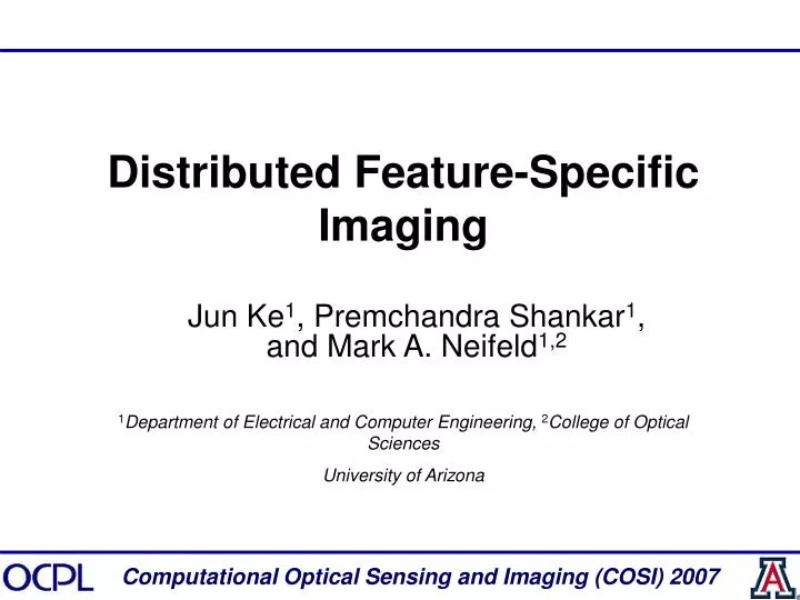
Distributed Feature-Specific Imaging. Jun Ke 1 , Premchandra Shankar 1 , and Mark A. Neifeld 1,2. 1 Department of Electrical and Computer Engineering, 2 College of Optical Sciences University of Arizona. Computational Optical Sensing and Imaging (COSI) 2007. Outline. Motivation

E N D
Distributed Feature-Specific Imaging Jun Ke1, Premchandra Shankar1, and Mark A. Neifeld1,2 1Department of Electrical and Computer Engineering, 2College of Optical Sciences University of Arizona Computational Optical Sensing and Imaging (COSI) 2007
Outline • Motivation • Distributed feature-specific imaging system • System performance – reconstruction error & lifetime • Experimental result • Conclusion COSI2007
Background noise n post processing object x measured image x+n collected irradiance reconstruction reconstruction conventional imager noise n post processing object x estimated feature Fx+n feature specific imager collected irradiance Conventional imaging : Feature-specific imaging (FSI) : • Projections: PCA, DCT and Hadamard, etc. COSI2007
Motivation Imager 1 Imager 1 n Imager 2 n Imager 2 n n Imager K Object:x Imager K Object:x n n Base station Base station Characteristics Distributed conventional imaging (DCI): Distributed feature-specific imaging (DFSI): # of measurement ←Large Small→ Complexity ←High Low→ Redundancy ←High Low→ Size/Weight/Power ←High Low→ Bandwidth ←High Low→ Lifetime ←Short Long→ • k = 1 → FSI → m = F x + n • k > 1 → DFSI → mk = (FkGk-1) Gkx + nk= Fkx + n • Gk ~ geometric transform for the kth imager. COSI2007
Feature-specific Imaging Architecture Programmable Mask Single Photo-Detector Noisy Measurement S mi = fi x + n i=1, …, L n Object: x Imaging Optics Light Collection Optics Fixed Mask n Noisy Measurements S mi = fi x + n, i=1, …, L L – Detector Array Object:x Imaging m-Optics Sequential FS imager: • Noise variance is proportional to Lσ02/T0 . Parallel FS imager: • Noise variance is proportional to σ02/T0. COSI2007
System Performance – Reconstruction Error Object examples (32x32): • Feature measurements: where, • is the total # of features • For k imager DFSI, features are measured by each imager. • Wiener operator is used for reconstruction: where, • Reconstructed object: • RMSE: COSI2007
System Performance – Reconstruction Error M = total # of features M = total # of features • There is a minimum RMSE for each curve. • Parallel FSI is better than sequential FSI in term of RMSE. • PCA reaches minimum using small number of features. • PCA has the best performance when # of features is small. • Hadamard has the best performance when # of features is large. COSI2007
System Performance – Reconstruction Error high noise moderate noise low noise As k increases, • System collected photons increases • # of features per imager decrease • Photons per feature increases • RMSE reduces Using more imagers will increase fidelity • When noise is high, PCA and Hadamard projections have similar performances • When noise is moderate or low, Hadamard produces the smallest minimum RMSE • Generally, Hadamard projection is the best candidate for noisy environment. COSI2007
System Performance – Lifetime Imager 1 DCI: DFSI: N M/k n Imager 2 M/k Imager 1 N N M/k n n M/k Imager 2 N Imager K Object:x Object:x n M/k N N n M/k Imager K n Base station Base station • Lifetime ~ total # of data transmitted before energy runs out / # of data in each transmission • Normalized lifetime in DFSI: ~ Lifetime of DFSI / Lifetime of conventional imaging system = N/(M/k) • Compression has not been considered in both systems COSI2007
System Performance – Lifetime k Normalized lifetime with different projections and different number of imagers k: • Lifetime reduces as RMSE performance requirement is higher. • Lifetime is enlarged as more imagers are used. • With non-strict RMSE requirement, DFSI using PCA has the longest lifetime. • With strict requirement of RMSE, DFSI using Hadamard is the best option. Generally, DFSI with PCA present the best performance in term of lifetime. COSI2007
Experiment σ0 = 10-3 1200 Hadamard features original object k = 1,rmse=0.44 k = 2,rmse=0.18 k = 3,rmse=0.12 k = 4,rmse=0.10 k = 5,rmse=0.09 • There is a minimum RMSE for each curve • RMSE reduces as K increases. COSI2007
Conclusion • DFSI preserves FSI properties. • DFSI has better performance compared with FSI • Hadamard is the best projectionin term of reconstruction error. • PCA is the best projection in term of system lifetime. COSI2007
Experiment - result σ0 = 10-4, Hadamard 600 features • Block-wise data testing • Random projection has the biggest RMSE • PCA achieves minimum RMSE quick • Hadamard performs better with more features COSI2007