Download
1 / 39
390 likes | 478 Views
Explore the theoretical foundations of communication limits by delving into entropy, mutual information, and channel capacity theories. Understand how they impact transmission rates and error probabilities in various channel types.

E N D
Lecture-2: Limits of Communication • Problem Statement: Given a communication channel (bandwidth B), and an amount of transmit power, what is the maximum achievable transmission bit-rate (bits/sec), for which the bit-error-rate is (can be) sufficiently (infinitely) small ? - Shannon theory (1948) - Recent topic: MIMO-transmission (e.g. V-BLAST 1998, see also Lecture-1) Module-3 Transmission Marc Moonen Lecture-2 Limits of Communication K.U.Leuven-ESAT/SISTA
Overview • `Just enough information about entropy’ (Lee & Messerschmitt 1994) self-information, entropy, mutual information,… • Channel Capacity (frequency-flat channel) • Channel Capacity (frequency-selective channel) example: multicarrier transmission • MIMO Channel Capacity example: wireless MIMO Module-3 Transmission Marc Moonen Lecture-2 Limits of Communication K.U.Leuven-ESAT/SISTA
`Just enough information about entropy’(I) • Consider a random variable X with sample space (`alphabet’) • Self-information in an outcome is defined as where is probability for(Hartley 1928) • `rare events (low probability) carry more information than common events’ `self-information is the amount of uncertainty removed after observing .’ Module-3 Transmission Marc Moonen Lecture-2 Limits of Communication K.U.Leuven-ESAT/SISTA
`Just enough information about entropy’(II) • Consider a random variable X with sample space (`alphabet’) • Average information or entropy in X is defined as because of the log, information is measured in bits Module-3 Transmission Marc Moonen Lecture-2 Limits of Communication K.U.Leuven-ESAT/SISTA
`Just enough information about entropy’ (III) • Example: sample space (`alphabet’) is {0,1} with entropy=1 bit if q=1/2 (`equiprobable symbols’) entropy=0 bit if q=0 or q=1 (`no info in certain events’) H(X) 1 q 0 1 Module-3 Transmission Marc Moonen Lecture-2 Limits of Communication K.U.Leuven-ESAT/SISTA
`Just enough information about entropy’ (IV) • `Bits’ being a measure for entropy is slightly confusing (e.g. H(X)=0.456 bits??), but the theory leads to results, agreeing with our intuition (and with a `bit’ again being something that is either a `0’ or a `1’), and a spectacular theorem • Example: alphabet with M=2^n equiprobable symbols : -> entropy = n bits i.e. every symbol carries n bits Module-3 Transmission Marc Moonen Lecture-2 Limits of Communication K.U.Leuven-ESAT/SISTA
`Just enough information about entropy’ (V) • Consider a second random variable Y with sample space (`alphabet’) • Y is viewed as a `channel output’, when X is the `channel input’. • Observing Y, tells something about X: is the probability for after observing Module-3 Transmission Marc Moonen Lecture-2 Limits of Communication K.U.Leuven-ESAT/SISTA
`Just enough information about entropy’ (VI) • Example-1 : • Example-2 : (infinitely large alphabet size for Y) decision device noise 00 01 10 11 00 01 10 11 X Y + noise 00 01 10 11 X Y + Module-3 Transmission Marc Moonen Lecture-2 Limits of Communication K.U.Leuven-ESAT/SISTA
`Just enough information about entropy’(VII) • Average-information or entropy in X is defined as • Conditional entropy in X is defined as Conditional entropy is a measure of the average uncertainty about the channel input X after observing the output Y Module-3 Transmission Marc Moonen Lecture-2 Limits of Communication K.U.Leuven-ESAT/SISTA
`Just enough information about entropy’(VIII) • Average information or entropy in X is defined as • Conditional entropy in X is defined as • Average mutual information is defined as I(X|Y) is uncertainty about X that is removed by observing Y Module-3 Transmission Marc Moonen Lecture-2 Limits of Communication K.U.Leuven-ESAT/SISTA
Channel Capacity (I) • Average mutual information is defined by -the channel, i.e. transition probabilities -but also by the input probabilities • Channel capacity(`per symbol’ or `per channel use’) is defined as the maximum I(X|Y) for all possible choices of • A remarkably simple result: For a real-valued additive Gaussian noise channel, and infinitely large alphabet for X (and Y), channel capacity is signal (noise) variances Module-3 Transmission Marc Moonen Lecture-2 Limits of Communication K.U.Leuven-ESAT/SISTA
Channel Capacity (II) • A remarkable theorem (Shannon 1948): With R channel uses per second, and channel capacity C, a bit stream with bit-rate C*R (=capacity in bits/sec) can be transmitted with arbitrarily low probability of error = Upper bound for system performance ! Module-3 Transmission Marc Moonen Lecture-2 Limits of Communication K.U.Leuven-ESAT/SISTA
Channel Capacity (II) • For a real-valued additive Gaussian noise channel, and infinitely large alphabet for X (and Y), the channel capacity is • For a complex-valued additive Gaussian noise channel, and infinitely large alphabet for X (and Y), the channel capacity is Module-3 Transmission Marc Moonen Lecture-2 Limits of Communication K.U.Leuven-ESAT/SISTA
Channel Capacity (III) Information I(X|Y) conveyed by a real-valued channel with additive white Gaussian noise, for different input alphabets, with all symbols in the alphabet equally likely (Ungerboeck 1982) Module-3 Transmission Marc Moonen Lecture-2 Limits of Communication K.U.Leuven-ESAT/SISTA
Channel Capacity (IV) Information I(X|Y) conveyed by a complex-valued channel with additive white Gaussian noise, for different input alphabets, with all symbols in the alphabet equally likely(Ungerboeck 1982) Module-3 Transmission Marc Moonen Lecture-2 Limits of Communication K.U.Leuven-ESAT/SISTA
Channel Capacity (V) This shows that, as long as the alphabet is sufficiently large, there is no significant loss in capacity by choosing a discrete input alphabet, hence justifies the usage of such alphabets ! The higher the SNR, the larger the required alphabet to approximate channel capacity Module-3 Transmission Marc Moonen Lecture-2 Limits of Communication K.U.Leuven-ESAT/SISTA
Channel Capacity (frequency-flat channels) • Up till now we considered capacity `per symbol’ or `per channel use’ • A continuous-time channel with bandwidth B (Hz) allows 2B (per second) channel uses (*), i.e. 2B symbols being transmitted per second, hence capacity is (*) This is Nyquist criterion `upside-down’ (see also Lecture-3) received signal (noise) power Module-3 Transmission Marc Moonen Lecture-2 Limits of Communication K.U.Leuven-ESAT/SISTA
s(t) r(t)=Ho.s(t)+n(t) Ho H(f) channel Ho f B -B Channel Capacity (frequency-flat channels) • Example: AWGN baseband channel (additive white Gaussian noise channel) + here n(t) Module-3 Transmission Marc Moonen Lecture-2 Limits of Communication K.U.Leuven-ESAT/SISTA
s(t) r(t)=Ho.s(t)+n(t) Ho channel Channel Capacity (frequency-flat channels) • Example: AWGN passband channel passband channel with bandwidth B accommodates complex baseband signal with bandwidth B/2 (see Lecture-3) + n(t) H(f) Ho f x x+B Module-3 Transmission Marc Moonen Lecture-2 Limits of Communication K.U.Leuven-ESAT/SISTA
Channel Capacity (frequency-selective channels) • Example: frequency-selective AWGN-channel received SNR is frequency-dependent! s(t) R(f)=H(f).S(f)+N(f) + H(f) channel H(f) n(t) f -B B Module-3 Transmission Marc Moonen Lecture-2 Limits of Communication K.U.Leuven-ESAT/SISTA
Channel Capacity (frequency-selective channels) • Divide bandwidth into small bins of width df, such that H(f) is approx. constant over df • Capacity is optimal transmit power spectrum? B 0 H(f) f -B B Module-3 Transmission Marc Moonen Lecture-2 Limits of Communication K.U.Leuven-ESAT/SISTA
Channel Capacity (frequency-selective channels) Maximize subject to solution is `Water-pouring spectrum’ Available Power L B area Module-3 Transmission Marc Moonen Lecture-2 Limits of Communication K.U.Leuven-ESAT/SISTA
Channel Capacity (frequency-selective channels) Example : multicarrier modulation available bandwidth is split up into different `tones’, every tone has a QAM-modulated carrier (modulation/demodulation by means of IFFT/FFT). In ADSL, e.g., every tone is given (+/-) the same power, such that an upper bound for capacity is (white noise case) (see Lecture-7/8) Module-3 Transmission Marc Moonen Lecture-2 Limits of Communication K.U.Leuven-ESAT/SISTA
MIMO Channel Capacity (I) • SISO =`single-input/single output’ • MIMO=`multiple-inputs/multiple-outputs’ • Question: we usually think of channels with one transmitter and one receiver. Could there be any advantage in using multiple transmitters and/or receivers (e.g. multiple transmit/receive antennas in a wireless setting) ??? • Answer: You bet.. Module-3 Transmission Marc Moonen Lecture-2 Limits of Communication K.U.Leuven-ESAT/SISTA
N1 X1 Y1 + + X2 Y2 N2 MIMO Channel Capacity (II) • 2-input/2-output example A B C D Module-3 Transmission Marc Moonen Lecture-2 Limits of Communication K.U.Leuven-ESAT/SISTA
MIMO Channel Capacity (III) Rules of the game: • P transmitters means that the same total power is distributed over the available transmitters (no cheating) • Q receivers means every receive signal is corrupted by the same amount of noise (no cheating) Noises on different receivers are often assumed to be uncorrelated (`spatially white’), for simplicity Module-3 Transmission Marc Moonen Lecture-2 Limits of Communication K.U.Leuven-ESAT/SISTA
N1 X1 Y1 + + first example/attempt X2 Y2 N2 MIMO Channel Capacity (IV) 2-in/2-out example, frequency-flat channels Ho 0 0 Ho Module-3 Transmission Marc Moonen Lecture-2 Limits of Communication K.U.Leuven-ESAT/SISTA
MIMO Channel Capacity (V) 2-in/2-out example, frequency-flat channels • corresponds to two separate channels, each with input power and additive noise • total capacity is • room for improvement... Module-3 Transmission Marc Moonen Lecture-2 Limits of Communication K.U.Leuven-ESAT/SISTA
N1 X1 Y1 + + X2 Y2 N2 MIMO Channel Capacity (VI) 2-in/2-out example, frequency-flat channels Ho Ho second example/attempt -Ho Ho Module-3 Transmission Marc Moonen Lecture-2 Limits of Communication K.U.Leuven-ESAT/SISTA
MIMO Channel Capacity (VII) A little linear algebra….. Matrix V’ Module-3 Transmission Marc Moonen Lecture-2 Limits of Communication K.U.Leuven-ESAT/SISTA
MIMO Channel Capacity (VIII) A little linear algebra…. (continued) • Matrix V is `orthogonal’ (V’.V=I) which means that it represents a transformation that conserves energy/power • Use as a transmitter pre-transformation • then (use V’.V=I) ... Dig up your linear algebra course notes... Module-3 Transmission Marc Moonen Lecture-2 Limits of Communication K.U.Leuven-ESAT/SISTA
+ + + + MIMO Channel Capacity (IX) • Then… X1 N1 X^1 A Y1 V11 V12 B V21 C X^2 Y2 V22 D transmitter X2 N2 channel receiver Module-3 Transmission Marc Moonen Lecture-2 Limits of Communication K.U.Leuven-ESAT/SISTA
MIMO Channel Capacity (X) • corresponds to two separate channels, each with input power , output power and additive noise • total capacity is 2x SISO-capacity! Module-3 Transmission Marc Moonen Lecture-2 Limits of Communication K.U.Leuven-ESAT/SISTA
MIMO Channel Capacity (XI) • Conclusion: in general, with P transmitters and P receivers, capacity can be increased with a factor up to P (!) • But: have to be `lucky’ with the channel (cfr. the two `attempts/examples’) • Example : V-BLAST (Lucent 1998) up to 40 bits/sec/Hz in a `rich scattering environment’ (reflectors, …) Module-3 Transmission Marc Moonen Lecture-2 Limits of Communication K.U.Leuven-ESAT/SISTA
MIMO Channel Capacity (XII) • General I/O-model is : • every H may be decomposed into this is called a `singular value decompostion’, and works for every matrix (check your MatLab manuals) orthogonal matrix V’.V=I orthogonal matrix U’.U=I diagonal matrix Module-3 Transmission Marc Moonen Lecture-2 Limits of Communication K.U.Leuven-ESAT/SISTA
MIMO Channel Capacity (XIII) With H=U.S.V’, • V is used as transmitter pre-tranformation (preserves transmit energy) and • U’ is used as a receiver transformation (preserves noise energy on every channel) • S=diagonal matrix, represents resulting, effectively `decoupled’ (SISO) channels • Overall capacity is sum of SISO-capacities • Power allocation over SISO-channels (and as a function of frequency) : water pouring Module-3 Transmission Marc Moonen Lecture-2 Limits of Communication K.U.Leuven-ESAT/SISTA
MIMO Channel Capacity (XIV) Reference: G.G. Rayleigh & J.M. Cioffi `Spatio-temporal coding for wireless communications’ IEEE Trans. On Communications, March 1998 Module-3 Transmission Marc Moonen Lecture-2 Limits of Communication K.U.Leuven-ESAT/SISTA
Assignment 1 (I) • 1. Self-study material Dig up your favorite (?) signal processing textbook & refresh your knowledge on -discrete-time & continuous time signals & systems -signal transforms (s- and z-transforms, Fourier) -convolution, correlation -digital filters ...will need this in next lectures Module-3 Transmission Marc Moonen Lecture-2 Limits of Communication K.U.Leuven-ESAT/SISTA
Assignment 1 (II) • 2. Exercise (MIMO channel capacity) Investigate channel capacity for… -SIMO-system with 1 transmitter, Q receivers -MISO-system with P transmitters, 1 receiver -MIMO-system with P transmitters, Q receivers P=Q (see Lecture 2) P>Q P<Q Module-3 Transmission Marc Moonen Lecture-2 Limits of Communication K.U.Leuven-ESAT/SISTA