Download
1 / 27
490 likes | 995 Views
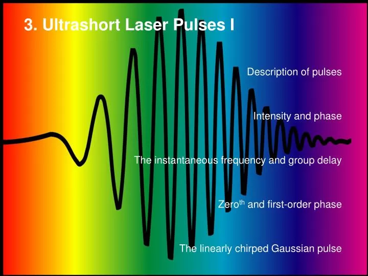
3. Ultrashort Laser Pulses I. Description of pulses Intensity and phase The instantaneous frequency and group delay Zero th and first-order phase The linearly chirped Gaussian pulse. An ultrashort laser pulse has an intensity and phase vs. time.

E N D
3. Ultrashort Laser Pulses I • Description of pulses • Intensity and phase • The instantaneous frequency and group delay • Zeroth and first-order phase • The linearly chirped Gaussian pulse
An ultrashort laser pulse has an intensity and phase vs. time. Neglecting the spatial dependence for now, the pulse electric field is given by: Intensity Phase Carrier frequency A sharply peaked function for the intensity yields an ultrashort pulse. The phase tells us the color evolution of the pulse in time.
The real and complex pulse amplitudes Removing the 1/2, the c.c., and the exponential factor with the carrier frequency yields the complex amplitude,E(t), of the pulse: This removes the rapidly varying part of the pulse electric field and yields a complex quantity, which is actually easier to calculate with. is often called the real amplitude,A(t), of the pulse.
The Gaussian Pulse For almost all calculations, a good first approximation for any ultrashort pulse is the Gaussian pulse (with zero phase). • where tFWHM is the full-width-half-maximum of the intensity. • The intensity is:
Intensity vs. amplitude The phase of this pulse is constant, (t) = 0, and is not plotted. The intensity of a Gaussian pulse is √2 shorter than its real amplitude. This factor varies from pulse shape to pulse shape.
Calculating the Intensity and the Phase It’s easy to go back and forth between the electric field and the intensity and phase. The intensity: I(t) = |E(t)|2 The phase: E(ti) Im √I(ti) f(ti) Equivalently, Re f(t) = Im{ ln[E(t)] }
The Fourier Transform • To think about ultrashort laser pulses, the Fourier Transform is essential. We always perform Fourier transforms on the pulse electric field.
The frequency-domain electric field • The frequency-domain equivalents of the intensity and phase are the spectrum and spectral phase. • Fourier-transforming the pulse electric field: yields: Note that f and j are different! The frequency-domain electric field has positive- and negative-frequency components.
The complex frequency-domain pulse field Since the negative-frequency component contains the same infor-mation as the positive-frequency component, we usually neglect it. We also center the pulse on its actual frequency, not zero. Thus, the most commonly used complex frequency-domain pulse field is: Thus, the frequency-domain electric field also has an intensity and phase. S is the spectrum, and j is the spectral phase.
We usually use just this component. The Spectrum with and without the carrier frequency • Fourier transforming E(t) and E(t) yield different functions.
The Spectrum and Spectral Phase • The spectrum and spectral phase are obtained from the frequency-domain field the same way as the intensity and phase are from the time-domain electric field. or
Transforming between wavelength and frequency. • The spectrum and spectral phase vs. frequency differ from the spectrum and spectral phase vs. wavelength. Because the energy is the same, whether we integrate the spectrum over frequency or wavelength: Changing variables:
The spectrum and spectral phase vs. wavelength and frequency • Example: A Gaussian spectrum with a linear phase vs. frequency vs. Frequency vs. Wavelength Note the different shapes of the spectrum when plotted vs. wavelength and frequency.
The Instantaneous frequency The temporal phase,(t), contains frequency-vs.-time information. The pulse instantaneous angular frequency, inst(t), is defined as: This is easy to see. At some time, t, consider the total phase of the wave. Call this quantity 0: Exactly one period, T, later, the total phase will (by definition) increase to 0 + 2p: where (t+T) is the slowly varying phase at the time,t+T. Subtracting these two equations:
Instantaneous frequency (cont’d) Dividing by T and recognizing that 2π/T is a frequency, call it inst(t): inst(t) = 2π/T = 0 – [(t+T) – (t)] / T But Tis small, so [(t+T)–(t)] /T is the derivative, d /dt. So we’re done! Usually, however, we’ll think in terms of the instantaneous frequency, inst(t), so we’ll need to divide by 2: inst(t) = 0 – [d/dt] / 2 While the instantaneous frequency isn’t always a rigorous quantity, it’s fine for ultrashort pulses, which have broad bandwidths.
Group delay While the temporal phase contains frequency-vs.-time information, the spectral phase contains time-vs.-frequency information. So we can define the group delay vs. frequency, tgr(w), given by: tgr(w) = d / d A similar derivation to that for the instantaneous frequency can show that this definition is reasonable. Also, we’ll typically use this result, which is a real time (the rad’s cancel out), and never d/d, which isn’t. Always remember that tgr(w) is not the inverse of inst(t).
Phase Wrapping and Unwrapping • Technically, the phase ranges from –p to p. But it often helps to “unwrap” it. This involves adding or subtracting 2p whenever there’s a p phase jump. • Example: a pulse with quadratic phase Unwrapped phase Wrapped phase The main reason for unwrapping the phase is aesthetics.
Phase-Blanking • When the intensity is zero, the phase is meaningless. • When the intensity is nearly zero, the phase is nearly meaningless. • Phase-blanking involves simply not plotting the phase when the intensity is close to zero. Without phase blanking With phase blanking The only problem with phase-blanking is that you have to decide the intensity level below which the phase is meaningless.
Phase Taylor Series expansions We can write a Taylor series for the phase, f(t), about the timet = 0: where is related to the instantaneous frequency. where only the first few terms are typically required to describe well-behaved pulses. Of course, we’ll consider badly behaved pulses, which have higher-order terms in (t). Expanding the phase in time is not common because it’s hard to measure the intensity vs. time, so we’d have to expand it, too.
Frequency-domain phase expansion It’s more common to write a Taylor series for (): where is the group delay! is called the “group-delay dispersion.” As in the time domain, only the first few terms are typically required to describe well-behaved pulses. Of course, we’ll consider badly behaved pulses, which have higher-order terms in ().
Zeroth-order Phase: The Absolute Phase • The absolute phase is the same in both the time and frequency domains. • An absolute phase of p/2 will turn a cosine carrier wave into a sine. • It’s usually irrelevant, unless the pulse is only a cycle or so long. Different absolute phases for a single-cycle pulse Different absolute phases for a four-cycle pulse Notice that the two four-cycle pulses look alike, but the three single-cycle pulses are all quite different.
First-order Phase in Frequency: A Shift in Time • By the Fourier-Transform Shift Theorem, Time domain Frequency domain Note that j1 does not affect the instantaneous frequency, but the group delay = j1.
First-order Phase in Time: A Frequency Shift • By the Inverse-Fourier-Transform Shift Theorem, Time domain Frequency domain Note that 1 does not affect the group delay, but the instantaneous frequency = –1.
Second-order Phase: The Linearly Chirped Pulse • A pulse can have a frequency that varies in time. This pulse increases its frequency linearly in time (from red to blue). In analogy to bird sounds, this pulse is called a "chirped" pulse.
The Linearly Chirped Gaussian Pulse • We can write a linearly chirped Gaussian pulse mathematically as: Gaussian amplitude Carrier wave Chirp Note that for b > 0, when t < 0, the two terms partially cancel, so the phase changes slowly with time (so the frequency is low). And when t > 0, the terms add, and the phase changes more rapidly (so the frequency is larger)
The Instantaneous Frequencyvs. time for a Chirped Pulse • A chirped pulse has: • where: • The instantaneous frequency is: • which is: • So the frequency increases linearly with time.
The Negatively Chirped Pulse • We have been considering a pulse whose frequency increases • linearly with time: a positively chirped pulse. • One can also have a negatively • chirped (Gaussian) pulse, whose • instantaneous frequency • decreases with time. • We simply allow b to be negative • in the expression for the pulse: • And the instantaneous frequency will decrease with time: