Download
1 / 39
390 likes | 400 Views
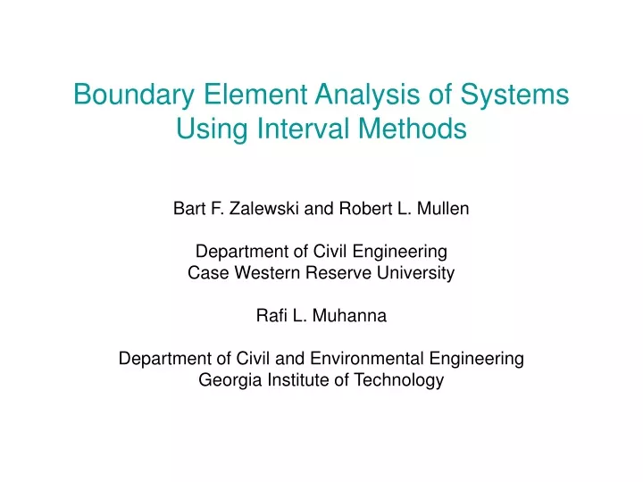
Boundary Element Analysis of Systems Using Interval Methods. Bart F. Zalewski and Robert L. Mullen Department of Civil Engineering Case Western Reserve University Rafi L. Muhanna Department of Civil and Environmental Engineering Georgia Institute of Technology. BEA.

E N D
Boundary Element Analysis of Systems Using Interval Methods Bart F. Zalewski and Robert L. Mullen Department of Civil Engineering Case Western Reserve University Rafi L. Muhanna Department of Civil and Environmental Engineering Georgia Institute of Technology
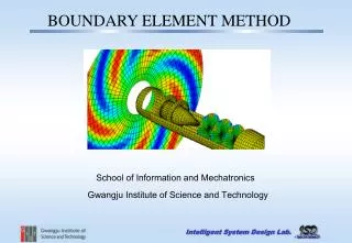
BEA Boundary Element Analysis (BEA) is a method for obtaining approximate solutions of partial differential equations. BEA is performed using transformation of the system’s domain variables to the variables on the boundaries of the system. BEA requires less meshing than finite element analysis and thus it is comparatively faster in generating or refining the mesh.
BEA (Cont.) The variable transformation is constructed using singular solutions of the governing partial differential equation. The transformed boundary integral equations are solved using collocation methods. Source points are located sequentially at all boundary nodes that map the domain variables such that they coincide to their nodal values.
BEA (Cont.) The following sources are a cause of error in BEA: Uncertainty in boundary conditions Uncertainty in the parameters of the system Errors in integration Errors in the solution of the resulting linear system of equations Discretization errors
Objective To explore the applications of interval concepts to boundary element methods Procedure To perform the boundary element analysis of Laplace equation considering interval uncertainties
Presentation Outline • Deterministic BEA of Laplace equation • Interval BEA • Truncation error • Integration error • Uncertain boundary conditions • Discretization error • Examples • Conclusion
Boundary Element Analysisof Laplace Equation The Laplace equation is: is the domain of the system is the boundary of the system , are the values at the boundary
Boundary Element Analysisof Laplace Equation (Cont.) Orthogonalization of Laplace equation with respect to a test function is performed to minimize the error due to approximation of the the exact solution of and :
Boundary Element Analysisof Laplace Equation (Cont.) Twice integrating by parts on the left side and considering and yields: is a source point (Brebbia 1992)
Boundary Element Analysisof Laplace Equation (Cont.) Before the application of boundary conditions the boundary is taken along . The boundary integral equation is integrated such that the source point is included on the circular boundary of radius , as :
Constant Boundary Element Discretization Any boundary can be discretized into boundary elements consisting of nodes, at which a value of either or is known, and also consisting of assumed polynomial shape functions between nodes.
Constant Boundary Element Discretization (Cont.) In this work one-noded boundary elements with constant shape functions are used, leading to the following discretization: and are vectors of nodal values is a vector of constant shape functions
Constant Boundary Element Discretization (Cont.) The discretized integral equation is written as: or in matrix form: Applying the boundary conditions, the system of linear equations is rearranged as:
Boundary Element Formulation and are fully populated non-symmetric matrices. The diagonal terms of the matrix are computed such that the matrix is singular. The diagonal terms of the matrix require special consideration since they contain singular integrals.
Interval Boundary Element Formulation The following are considered as interval quantities in the interval BEA analysis: Truncation error Integration error Uncertainty in boundary conditions Discretization error
Interval Boundary ElementFormulation (Cont.) Interval boundary element analysis is performed as: The equation is rearranged as: The interval linear system of equation can be solved by Matlab Interval Toolbox [MATLAB 6.5.1], which uses Newton-Krawczyk iteration.
Interval Boundary ElementFormulation (Cont.) The approximate value of the diagonal terms of the matrix is computed using the Taylor series expansion. In order to bound the integration error, the closed form solution of the improper integral of the diagonal terms is found, which is not necessarily in the domain of the actual problem.
Interval Boundary ElementFormulation (Cont.) If the domain of the improper integral is different than that of the problem, the remaining domain is integrated numerically using Taylor series expansion and the integration error found using the given error bound. If the domain of the improper integral is that of the problem, the difference between the closed form solution and the numerical integration is considered as integration error.
Taylor Series Expansion A function can be expressed as a polynomial using Taylor series expansion [Taylor, 1715]: where Any function can be integrated exactly as: where corresponds to the derivative of the function
Error Analysis on TaylorSeries Expansion is the series remainder as: Integrating the remainder yields:
Error Analysis on TaylorSeries Expansion (Cont.) The maximum truncation error is found: The approximate terms of the and matrices are computed as:
Integration Error The integration error can be represented by an interval variable. The real interval number is a closed set as: Then the bounds on the integration error are computed: Alternative series may yield sharper bounds depending on the partial differential equation considered.
Uncertainty in Boundary Conditions Considering uncertainty in boundary conditions results in interval vectors and . Parameterization of the rows of and matrices is considered to obtain sharp results and the system is solved as:
Discretization Error In the analysis of the discretiztion error, we will look for interval bounded unknown functions that will satisfy the continuous problem.
Discretization Error (Cont.) The boundary is subdivided into elements. For each element, we will seek the interval values and that bound the functions and over an element such that:
Discretization Error (Cont.) The integral of the product will be expanded to the product of the interval value of or and the interval bounds of the integral of the singular solution over the element for all values of : if has the same sign over the element.
Discretization Error (Cont.) If not, the integration domain is subdivided into portions that have the same sign for . Then the integral is replaced by interval bounds: Thus, the interval bounds on the solution can be expressed as a generalized interval system of linear equations. For sharp bounds, the parametric dependence of each row of the or matrices on must be included in the solution of the interval system.
Examples The first example uses interval BEA to bound the solution to Laplace equation in the presence of truncation and integration errors. Four point integration method based on a Taylor series is used to develop interval terms in matrices. Boundary Conditions: u1=0, q2=0, q3=0, u4=50, q5=0, q6=0 1:2 ratio
Examples (Cont.) Results:
Examples (Cont.) The second example is a demonstration of the interval treatment of uncertain boundary conditions. Boundary Conditions: u1=[0,1], q2=0, q3=0, u4=[1,2], q5=0, q6=0 1:1 ratio
Examples (Cont.) Results:
Examples (Cont.) The third example obtains the bounds on discretization error for the BEA of the Laplace equation. Interval bounds of the and matrices are constructed by moving the point over the domain of an element. Boundary Conditions: Boundary Conditions: Boundary Conditions: u1=0 u1=0 u1=0 u5=1 q2=0 q2=0 q2=0 q6=0 u3=1 q3=0 q3=0 q7=0 q4=0 u4=1 q4=0 q8=0 q5=0 q6=0 , 1:1 ratio 1:1 ratio 1:1 ratio
Examples (Cont.) Results:
Examples (Cont.) Results:
Examples (Cont.) Results:
Examples (Cont.) Results:
Conclusion In this work, new methods are presented to perform boundary element analysis in the presence of the truncation, integration and discretization errors as well as uncertain boundary conditions using interval methods. The examples presented demonstrate the potential of interval based boundary element methods to provide reliable engineering computations. Further work is needed to optimally solve the parametric form of the interval equations to advance interval based BEA to a truly reliable and efficient engineering analysis tool.
Acknowledgment The authors thank Dr. Mehdi Modares for his tremendous help throughout the present work.