Download

1 / 50
500 likes | 578 Views
High Performance Integration of Data Parallel File Systems and Computing. Zhenhua Guo. Outline. Introduction and Motivation Literature Survey Research Issues and Our Approaches Contributions. Traditional HPC Architecture vs. the Architecture of Data Parallel Systems. HPC Arch.

E N D
High Performance Integration of Data Parallel File Systems and Computing Zhenhua Guo PhD Thesis Proposal
Outline • Introduction and Motivation • Literature Survey • Research Issues and Our Approaches • Contributions
Traditional HPC Architecture vs. the Architecture of Data Parallel Systems HPC Arch. • Separate compute and storage • Advantages • Separation of concerns • Same storage system can be mounted to multiple compute venues • Drawbacks • Bring data to compute data movement • Impose load on oversubscribed network • Data availability: RAID, Tape • Examples: TeraGrid • Usually run on high-profile servers • Data Parallel System Arch. • The same set of nodes for compute and storage • Designed for data parallel applications • Run on commodity hardware • Data availability: replication • Scheduling • bring compute to data • bring compute close to data Storage Cluster 2 Cluster 1
Data Parallel Systems • Google File System/MapReduce, Twister, Cosmos/Drayad, Sector/Sphere • MapReduce has quickly gained popularity • Google, Yahoo!, Facebook, Amazon EMR,… • Academic usage: data mining, log processing, … • Substantial research • MapReduce online, Map-Reduce-Merge, Hierarchical MapReduce … • Hadoop is an open source implementation of GFS and MapReduce • Killing features • Simplicity • Fault tolerance • Extensibility • Scalability
MapReduce Model • Input & Output: a set of key/value pairs • Two primitive operations • map: (k1,v1) list(k2,v2) • reduce: (k2,list(v2)) list(k3,v3) • Each map operation processes one input key/value pair and produces a set of key/value pairs • Each reduce operation • Merges all intermediate values (produced by map ops) for a particular key • Produce final key/value pairs • Operations are organized into tasks • Map tasks: apply map operation to a set of key/value pairs • Reduce tasks: apply reduce operation to intermediate key/value pairs • Each MapReduce job comprises a set of map and reduce (optional) tasks. • Use Google File System to store data • Optimized for large files and write-once-read-many access patterns • HDFS is an open source implementation • Can be extended to non key/value pair models
MapReduce Execution Overview Google File System Read input dataData locality Input file block 0 1 2 map tasks Stored locally Shuffle between map tasks and reduce tasks reduce tasks Stored in GFS Google File System
Hadoop Implementation Storage: HDFS - Files are split into blocks. - Each block has replicas. - All blocks are managed by central name node. Metadata mgmt. Task scheduler HDFS Name node MapReduce Job tracker Fault tolerance Replication mgmt. Block placement …… • Compute: MapReduce • - Each node has map and reduce slots- Tasks are scheduled totask slots • # of tasks <= # of slots Hadoop Hadoop …… Operating System Operating System task slot data block Worker node 1 Worker node N
Motivation • GFS/MapReduce (Hadoop) is our research target • Overall, MapReduce performs well for pleasantly parallel applications • Want a deep understanding of its performance for different configurations and environments • Observed inefficiency (thus degraded performance) that can be improved • For state-of-the-art schedulers, data locality is not optimal • Fixed task granularity ⇒ poor load balancing • Simple algorithms to trigger speculative execution • Low resource utilization when # of tasks is less than # of slots • How to build MapReduce across multiple grid clusters
Outline • Motivation • Literature Survey • Research Issues and Our Approaches • Contributions
Storage • Storage • Distributed Parallel Storage System (DPSS): disk-based cache over WAN to isolate apps and tertiary archive storage systems • Storage Resource Broker (SRB): unified APIs to heterogeneous data sources; catalog • DataGrid: a set of sites are federated to store large data sets. • Data staging and replication management • GridFTP: High-performance data movement • Reliable File Transfer, Replication Location Service, Data Replication Service • Stork: treat data staging as jobs, support many storage systems and transport protocols. • Parallel File System • Network File System, Lustre (used by IU data capacitor), General Purpose File System (GPFS) (used by IU Bigred), Parallel Virtual File System (PVFS) • Google File System: non-POSIX • Other storage systems • Object store: Amazon S3, OpenStack Swift • Key/Value store: Redis, Riak, Tokyo Cabinet • Document-oriented store: Mongo DB, Couch DB • Column family: Bigtable/Hbase, Cassandra
Traditional Job Scheduling • Use task graph to represent dependency: • find a map from graph nodes to physical machines • Bag-of-Tasks: • Assume tasks of a job are independent. Heuristics: MinMin, MaxMin, Suffrage • Batch scheduler • Portable Batch System (PBS), Load Sharing Facility (LSF), LoadLeveler, and Simple Linux Utility for Resource Management (SLURM) • Maintains job queue and allocates compute resources to jobs (no data affinity) • Gang scheduling • Synchronizes all processes of a job for simultaneous scheduling • Co-scheduling • Communication-driven, coordinated by passing messages • Dynamic coscheduling, spin block, Periodic Boost, … • HYBRID: combine gang scheduling and coscheduling • Middleware • Condor: harness idle workstations to do useful computation • BOINC: volunteer computing • Globus: grid computing
MapReduce-related • Improvement of vanilla MapReduce • Delay scheduling: improve data locality • Largest Approximate Time to End: a better metric to make decisions about when/where to run spec. tasks • Purlieus: optimize VM provisioning in cloud for MapReduce apps • Most of my work falls into this category • Enhancements to MapReduce model • Iterative MapReduce: Haloop, Twister @IU, Spark • Map-Reduce-Merge: enable processing heterogeneous data sets • MapReduce online: online aggregation, and continuous queries • Alternative models • Dryad: use Direct Acyclic Graph to represent job
Outline • Motivation • Literature Survey • Research Issues and Our Approaches • Contributions
Research Objectives • Deploy data parallel system Hadoop to HPC clusters • Many HPC clusters exist already (e.g. TeraGrid/XSEDE, FutureGrid) • Evaluate performance – Hadoop and storage systems • Improve data locality • Analyze relationship between system factors and data locality • Analyze the optimality/non-optimality of existing schedulers • Propose scheduling algorithm that gives optimal data locality • Investigate task granularity • Analyze the drawbacks of fixed task granularity • Propose algorithms to dynamically adjust task granularity at runtime • Investigate resource utilization and speculative execution • Explore low resource utilization and inefficiency of running speculative tasks • Propose algorithms to allow running tasks to harness idle resources • Propose algorithms to make smarter decisions about the execution of speculative tasks • HeterogeneityAware MapReduce scheduling • HMR: Build a unified MapReduce cluster across multiple grid clusters • Minimize data IO time with real-time network information
Performance Evaluation - Hadoop • Investigate following factors • # of nodes, # of map slots per node, the size of input data • Measure job execution time and efficiency • Observations • Increase # of map slots • more tasks run concurrently • average task run time is increased • job run time is decreased • efficiency is decreased (overhead is increased) • turning point: beyond it, job runtime is not improved much • Vary # of nodes, the size of input data
Performance Evaluation – Importance of data locality • Measure how important data locality is to performance • Developed random scheduler: schedule tasks based on user-specified randomness • Conduct experiments for single-cluster, cross-cluster and HPC-style setup Single cluster Cross cluster HPC-style MapReduce HDFS Cluster B Cluster A MapReduce HDFS Percent of slowdown (%) MapReduce Cluster A Cluster B HDFS Cluster A Number of slots per node (1) w/ high inter-cluster BW (2) w/ low inter-cluster BW (a) Single-cluster (b) Cross-cluster and HPC-style • Data locality matters • Hadoop performs poorly with drastically heterogeneous network
Performance Evaluation - Storage Local Disk Network File System (NFS) One worker node. All data accesses are local through HDFS API Hadoop Distributed File System (HDFS) OpenStack Swift HDFS and Swift are not efficiently implemented.
Data Locality • “distance” between compute and data • Different levels: node-level, rack-level, etc. • For data-intensive computing, data locality is critical to reduce network traffic • Research questions • Evaluate how system factors impact data locality and theoretically deduce their relationship • Analyze state-of-the-art scheduling algorithms in MapReduce • Propose scheduling algorithm giving optimal data locality
Data Locality - Analysis • Theoretical deduction of relationship between system factors and data locality (for Hadoop scheduling) • Assumptions • Data are randomly placed across nodes • Idle slots are randomly chosen from all slots • For simplicity • Replication factor is 1 • # of slots on each node is 1 • The ratio of data local tasks
Data Locality – Experiment 1 • Measure the relationship between system factors and data locality and verify our simulation • y-axis: percent of map tasks that achieve data locality. better Number of tasks (log scale) Number of slots per node Replication factor Number of tasks (normal scale) Ratio of idle slots Num. of idle slots / num. of tasks (redraw e) Number of nodes Num. of idle slots / num. of tasks (redraw a)
Data Locality - Optimality • Problem: given a set of tasks and a set of idle slots, assign tasks to idle slots • Hadoop schedules tasks one by one • Consider one idle slot each time • Given an idle slot, schedules the task that yields the “best” data(from task queue) • Achieve local optimum; global optimum is not guaranteed • Each task is scheduled without considering its impact on other tasks • All idle slots need to be considered at once to achieve global optimum • We propose an algorithm which gives optimal data locality • Reformulate the problem: • Construct a cost matrix • Cell C(i. j) is the incurred cost if task Tiis scheduled to idle slot sj 0: if compute and data are co-located 1: otherwiseReflects data locality • Find an assignment to minimize the sum of cost • Found a similar mathematical problem: Linear Sum Assignment Problem (LSAP) • Convert the scheduling problem to LSAP (not directly mapped) • Proved the optimality C(i, j) =
Data Locality – Experiment 2 • Measure the performance superiority of our proposed algorithm • y-axis: performance improvement (%) over native Hadoop
Task Granularity • Each task of a parallel job processes some amount of data • Use input data size to represent task granularity • To decide the optimal granularity is non-trivial • Internal structure of input data • Operations applied to data • Hardware • Each map task processes one block of data • Block size is configurable (by default 64MB) • The granularities of all tasks of a job are the same • Drawbacks • Limit the maximum degree of concurrency: num. # of blocks • Load unbalancing • An assumption made by Hadoop: Same input data size ⇒ Similar processing timeMay not always hold • Example: easy and difficult puzzlesInput is similar (9 x 9 grid) while solving them requires drastically different amounts of time Tradeoffs
Task Granularity – Auto. Re-organization • Our approach: dynamically change task granularity at runtime • Adapt to the real status of systems • Non-application-specific • Minimize overhead of task re-organization (best effort) • Cope with single-job and multi-job scenarios • Bag of Divisible Tasks (vs. Bag of Tasks) • Proposed mechanisms • Task consolidation consolidate tasks T1, T2, …, Tnto T • Task splitting split task T to spawn tasks T1, T2, …, and Tm • When there are idle slots and no waiting tasks, split running tasks • For multi-job env, we prove Shortest-Job-First (SJF) strategy gives optimal job turnaround time*. (arbitrarily divisible work) (UI: unprocessed input data)
Task Granularity – Task Re-organization Examples * May change data locality
Task Granularity – Single-Job Experiment System: 64 nodes, 1 map slot per node (can run 64 tasks concurrently at most) Synthesized workload: Task execution time follows Gaussian distribution. Fix mean and vary coefficient ofvariance (CV) better better Trace-based workload: Based on Google Cluster Data(75% short tasks, 20% long tasks,5% medium tasks)
Task Granularity – Multi-Job Experiment M/G/s model: inter-arrival time follows exponential dist (inter-arrival time << job execution time) 100 jobs are generated. i) Task execution time is the same for a job (balanced load) ii) Job serial execution time is different (75% short jobs, 20% long jobs, 5% others) i) Task execution time is different. ii) Job serial execution time is the same (all jobs are equally long) The system is fully load until last “wave” of task execution
Hierarchical MapReduce • Motivation • Single user may have access to multiple clusters (e.g. FutureGrid + TeraGrid + Campus clusters) • They are under the control of different domains • Need to unify themto build MapReducecluster • Extend MapReduce toMap-Reduce-GlobalReduce • Components • Global job scheduler • Data transferer • Workload reporter/collector • Job manager Global controller Local cluster Local cluster
Heterogeneity Aware Scheduling – Future Work • Will focus on network heterogeneity • Collect real-time network throughput information • Scheduling of map tasks • Minimize task completion time based on • resource availability • data IO/transfer time (depending on network performance) • Scheduling of reduce tasks • Goal: balance load so that they complete simultaneously • data shuffling : impact IO time • key distribution at reducer side : impact computation time • Sum should be balanced: min{maxS – minS} (S is a scheduling) • Both scheduling problems are NP hard. • Will investigate heuristics that perform well • Data Replication • How to increase replication rate in heterogeneous env.
Resource Stealing • In Hadoop, each node has a number of map and reduce slots • Drawback: low resource utilization (for native MR apps) • Example: node A has 8 cores, and the number of map slots is 7 (leave one core for Hadoop daemons) • If one map task is assigned to it, only 1 core is fully utilized while other 6 cores keep idle • We propose Resource Stealing • Running tasks “steal” resources “reserved” for prospective tasks that will be assigned to idle slots • When new tasks are assigned, give back stolen resources proportionally • Enforced on a per-node basis • Resource Stealing is transparent to task/job scheduler • Can be used with any existing Hadoop scheduler • How to allocate idle resources to running tasks • Propose different strategies: Even, First-Come-Most, Shortest-Time-Left-Most, …
Resource Stealing - Example • Two nodes: Each has 5 cores, and 4 map slots. Idle slots: wasted resources Spawn more tasksto utilize idle cores
Speculative Execution • In large distributed systems, failure is the norm rather than the exception • Causes: hardware failure, software bug, process hang, … • Hadoop uses speculative execution to support fault tolerance • The master node monitors progresses of all tasks • Abnormally slow task start speculative tasks • Not consider whether it’s beneficial to run spec. tasks • Task A: 90% done, progress rate is 1 • Task B: 50% done, progress rate is 5 • A is too slow, start a speculative task A’ whose progress rate is 5 • A completes earlier than A’. Not useful to run A’ • We propose Benefit Aware Speculative Execution (BASE) • Estimate the benefit of starting speculative tasks, and only start them when it is beneficial • Aim to eliminate the execution of unnecessary speculative tasks
Outline • Motivation • Literature Survey • Research Issues and Our Approaches • Contributions
Contributions and Future Work • Conduct in-depth evaluation of data parallel systems • Propose improvements for various aspects of MapReduce/Hadoop • Data locality • Adjustment of task granularity • Resource utilization and Speculative Execution • Heterogeneity Aware • Conduct experiments to demonstrate the effectiveness of our approaches • Future work • Investigate network heterogeneity aware scheduling
Introduction • Data intensive computing • The Fourth Paradigm – Data deluge in many areas • Ocean science, ecological science, biology, astronomy … • Several terabytes of data are collected per day • Exascale computing • New challenges • Data management - bandwidth/core drops dramatically • Heterogeneity • Programming models and runtimes • Fault tolerance • Energy consumption
MapReduce Walkthrough - wordcount • wordcount: count the number of words in input data • More than one worker in the example groupby intermediate data final output (the, 1) reduce input (3 blocks) (the, 1) (weather, 1) the weather is good (is, 1) (good, 1) map reduce (the, 1) (is, 1) (is, 1) (is, 3) today is good map reduce (is, 1) (for, 1) good weather is good (weather, 1) (today, 1) (weather, 2) map reduce (today, 1) (weather, 1) (is, 1) (today, 1) (good, 1) ... (good, 1) (weather, 1) (good, 1) (good, 4) reduce (is, 1) (good, 1) (good, 1) (good, 1) reduce(key,values): result = 0For each count v in values: result += v emit (key, result) map(key,value): For each word w in value: emit (w, 1) (good, 1)
Data Locality – Optimality Linear Sum Assignment Problem: Given n items and n workers, the assignment of an item to a worker incurs a known cost. Each item is assigned to one worker and each worker only has one item assigned. Find the assignment that minimizes the sum of cost • T: num. of tasks; IS: num. of idle slots • T < IS: add IS-T dummy tasks, fill with a constant • T > IS: add T-IS dummy slots fill with a constant • Apply LSAP • Filter result Figure
Task Re-organization: Definitions • UI(T): unprocessed data of task T. • Task consolidation: consolidate tasks T1, T2, …, Tnto T • Task splitting: split task T to spawn tasks T1, T2, …, and Tm • Ways to split tasks are not unique b) and c) have the same makespan. Different number of task splittings
Task Re-organization: Research Issues • Metrics to optimize • Job turnaround time • The time between job submission and Job completion • Performance measurement from users’ POV • Different from overall system throughput • Makespan • Time to run all jobs (wait time + exec time) • Research issues • When to trigger task splitting • Which tasks should be split and how many new tasks to spawn • How to split • Scope • Single-job • Prior knowledge is unknown • Prior knowledge is known • Multi-job
Single-Job Aggressive Scheduling: Task Splitting w/o Prior Knowledge • When: tasks in queue < available slots • How • Evenly allocate available map slots until all are occupied • idle_map_slots / num_maptasks_in_queue • Split each block to sub-blocks, logically • Tasks processing one sub-block cannot be split # of unprocessed sub-blocks # of sub-blocks to be processed by each task after splitting # of new tasks to spawn
Task Splitting with Prior Knowledge • ASPK: Aggressive Scheduling with Prior Knowledge • When • # of tasks in queue < # of available slots • Prior knowledge • Estimated Remaining Exec Time (ERET) • Heuristics • Big tasks should be split first • Avoid splitting tasks that are small enough already • Favor dynamic threshold calculation • Split tasks when there is potential performance gain
Task splitting: Algorithm Details • Filter tasks with small ERET • Optimal Remaining Job Execution Time (ORJET) • total_ERET / num_slots • Compare ERET with ORJET • Adaptive • Sort tasks by ERET in descending order • Cluster tasks by ERET • One dimensional clustering: linear • Tasks with similar ERET are put into the same cluster • Go through clusters to calculate the gain • Given that splitting tasks in first i clusters is beneficial • Decide whether to also split tasks in cluster i+1 • For each task to split, evenly distribute unfinished work • # of new tasks: task_ERET / optimal_ERET(after splitting)
Task splitting: Example • Initial state • Running tasks: {100, 30, 80, 1, 10}; • # of idle slots: 8 • Filtering: {100, 30, 80, 10} • Sorting: {100, 80, 30, 10} • Clustering: { {100, 80}, {30}, {10} } • Iterating: • Split tasks in C1 and C2 • Tasks in C1: • Tasks in C2:
Task splitting: Multi-Job Scenarios • Constraints of Scheduling • r(t,i): amount of resource consumed by job i at time t • C: the capacity of a certain type of resource • Si: resource requirement of job i • Goal function • Assume jobs can be “arbitrarily” split into tasks • But not beyond minimum allowed task granularity
Short Job First Strategy (c) Continuous job exec. arrangement • Once F(J) is fixed, S(J) does NOT affect job turnaround time • Once a job start running, it should use all available resources • This problem can be solved by converting it to n jobs/1 machine problem • Shortest Job First (SJF) is optimal • Periodic scheduling: non-overlapping or overlapping
Task splitting: Experiment Environment • Simulation-based: mrsim • Environment setup
Hierarchical MapReduce • MaxMapperi: sum of map slots on clusteri • MapperRuni: # of running tasks on clusteri • MapperAvaili: # of available map slots on clusteri • NumCorei: # of CPU cores on clusteri • pi: max. num. of tasks concurrently running on each core • MaxMapperi = pi x NumCorei • MapperAvaili = MaxMapperi – MapperRuni • Weighti = (MAix Wi)/Sigmai=1…N(MAixWi) • Wi: static weight of each cluster (e.g. it can reflect compute power, or memory capacity) • NumMapJi = Weighti x NumMapJ