Download
1 / 21
210 likes | 320 Views
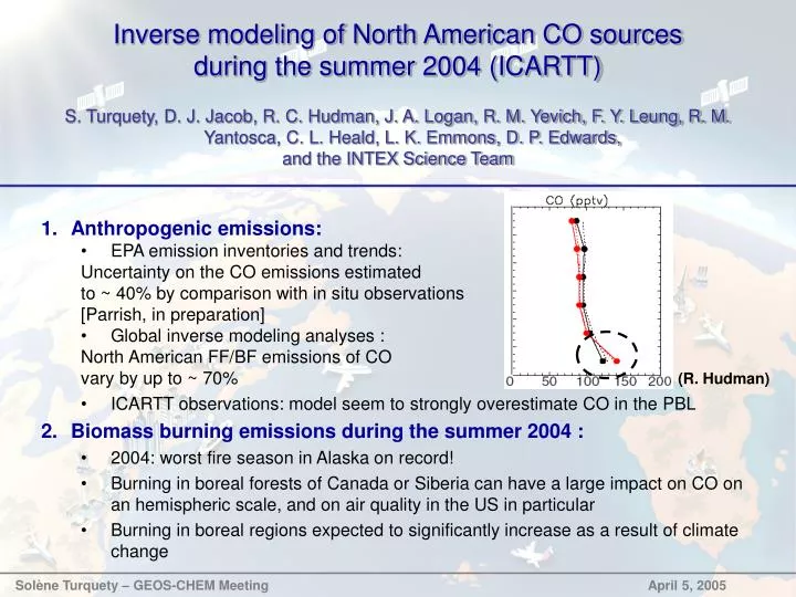
(R. Hudman). Sol ène Turquety – GEOS-CHEM Meeting April 5, 2005. Inverse modeling of North American CO sources during the summer 2004 (ICARTT)

E N D
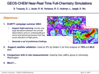
(R. Hudman) Solène Turquety – GEOS-CHEM Meeting April 5, 2005 • Inverse modeling of North American CO sources • during the summer 2004 (ICARTT) • S. Turquety, D. J. Jacob, R. C. Hudman, J. A. Logan, R. M. Yevich, F. Y. Leung, R. M. Yantosca, C. L. Heald, L. K. Emmons, D. P. Edwards, • and the INTEX Science Team • Anthropogenic emissions: • EPA emission inventories and trends: • Uncertainty on the CO emissions estimated • to ~ 40% by comparison with in situ observations • [Parrish, in preparation] • Global inverse modeling analyses : • North American FF/BF emissions of CO • vary by up to ~ 70% • ICARTT observations: model seem to strongly overestimate CO in the PBL • Biomass burning emissions during the summer 2004 : • 2004: worst fire season in Alaska on record! • Burning in boreal forests of Canada or Siberia can have a large impact on CO on an hemispheric scale, and on air quality in the US in particular • Burning in boreal regions expected to significantly increase as a result of climate change
Bottom-up inventory of the biomass burning emissions in North America during the summer 2004 Solène Turquety – GEOS-CHEM Meeting April 5, 2005 US National Interagency Coordination Center (NICC) Canadian Interagency Forest Fire Center (CIFFC) • Alaska: • > 2.6 million hectares burned • > 8 x 10-year average • Canada: • 15 x average area burned in Yukon Territory (60% of national total) • 6 x average in British Columbia
Biomass burning 2004: Strong signature during ICARTT Solène Turquety – GEOS-CHEM Meeting April 5, 2005
Bottom-up inventory of the biomass burning emissions in North America during the summer 2004 Solène Turquety – GEOS-CHEM Meeting April 5, 2005 MODIS hotspots Daily reports of the area burned from the NIFC A x 60% [W.M. Hao, FSL, Personal comm.] Emissions / unit area Emissions CO 2004 Derive emissions for 10 species, with 1x1 horizontal resolution: NOx, CO, lumped >= C4 alkanes, lumped >= C3 alkenes, acetone, methyl ethyl ketone, acetaldehyde, propane, formaldehyde, and ethane.
Bottom-up inventory of the biomass burning emissions in North America during the summer 2004 Alaska 2004 Logan and Yevich Total emissions CO (Tg) Canada Day since June 1st, 2004 Solène Turquety – GEOS-CHEM Meeting April 5, 2005 • Total emissions North America June 1st – August 31st =10.3 Tg CO • Alaska : 5.7 Tg CO 3 x climatology Logan and Yevich • Canada: 4.5 Tg CO 0.9 x climatology ; Yukon territory: 2.3 Tg CO 4.4 x clim.
Bottom-up inventory of the biomass burning emissions in North America during the summer 2004 Solène Turquety – GEOS-CHEM Meeting April 5, 2005 MOPITT Total CO – summer 2004 GEOS-CHEM Total CO x MOPITT AK (MOPITT – Model)/MOPITT • On average: Underestimate emissions by ~ 25% on average • Area burned? Uncertainty reports… • Emissions / unit area (fuel loads) ? • Injection heights?
Solène Turquety – GEOS-CHEM Meeting April 5, 2005 Importance of injection heights for the 2004 Alaskan-Yukon fires Use TOMS AI as an indicator of the altitude of the aerosol layer: Sensitivity as altitude of the aerosol layer (low sensitivity to the PBL)
Alaska – Yukon fires summer 2004 Total CO emissions Maximum TOMS AI Day since June 1st, 2004 Solène Turquety – GEOS-CHEM Meeting April 5, 2005 Importance of injection heights for the 2004 Alaskan-Yukon fires Pyro-convective cloud from aircraft – June 27, 2004 http://www.cpi.com/remsensing/midatm/smoke.html
Biomass burning 2004: Strong signature during ICARTT Obs. G. W. Sachse GEOS-CHEM NRT Solène Turquety – GEOS-CHEM Meeting April 4, 2005 Biomass burning plume sampled by the DC-8 on flight # 9 (July 18th) GEOS-CHEM NRT
Solène Turquety – GEOS-CHEM Meeting April 5, 2005 Importance of injection heights for the 2004 Alaskan-Yukon fires Compute 5-days trajectories w/ GEOS-4 from TOMS AI to calculate exposure to aerosols (K. Pickering, GSFC, http://croc.gsfc.nasa.gov/intex/) 850hPa 700hPa 500hPa
Vertical distribution 200mb 5 % Upper troposphere 400mb 55 % Free troposphere 40 % Boundary layer PBL Solène Turquety – GEOS-CHEM Meeting April 5, 2005 Importance of injection heights for the 2004 Alaskan-Yukon fires What are the implications for CO inversion? MOPITT Total CO July 17-19, 2004 GEOS-CHEM Total CO x MOPITT AK July 17-19, 2004 (MOPITT – Model)/MOPITT
Solène Turquety – GEOS-CHEM Meeting April 5, 2005 Importance of injection heights for the 2004 Alaskan-Yukon fires What are the implications for CO inversion? GEOS-CHEM BB CO 100 % BL x MOPITT AK GEOS-CHEM BB CO 100 % FT x MOPITT AK GEOS-CHEM BB CO 100 % UT x MOPITT AK
Solène Turquety – GEOS-CHEM Meeting April 5, 2005 Importance of injection heights for the 2004 Alaskan-Yukon fires What is the implications for long range transport? MOPITT Total CO July 22-24, 2004 GEOS-CHEM Total CO x MOPITT AK July 22-24, 2004 (MOPITT – Model)/MOPITT
Solène Turquety – GEOS-CHEM Meeting April 5, 2005 Importance of injection heights for the 2004 Alaskan-Yukon fires What are the implications for long range transport? GEOS-CHEM BB CO 100 % BL x MOPITT AK GEOS-CHEM BB CO 100 % FT x MOPITT AK GEOS-CHEM BB CO 100 % UT x MOPITT AK
AIRS CO for July 18 GEOS-CHEM NRT July 18 MOPITT CO for July 18 Inversion GEOS-CHEM Inversion A priori sources A posteriori sources A posteriori sources Solène Turquety – GEOS-CHEM Meeting April 5, 2005 Ongoing and future work • Using satellite observations to constrain the daily North American biomass burning emissions during the summer 2004 • Magnitude? • Injection height? (?) + TOMS AI? MISR ? Strong variability => daily inversion
AIRS CO GEOS-CHEM NRT MOPITT CO ^ GEOS-CHEM x Inversion A priori sources A posteriori sources Solène Turquety – GEOS-CHEM Meeting April 5, 2005 Ongoing and future work • Inverse modeling of North American anthropogenic emissions of CO using aircraft and satellite measurements (?) xa
Solène Turquety – GEOS-CHEM Meeting April 5, 2005 Ongoing and future work …
Ongoing and future work Observation vector: Observation error State vector: CO sources MOPITT observation Model simulation, with MOPITT AK applied Linear approximation: with K provides the sensitivity of the measurement to the source of interest. Calculated using a tagged CO simulation
Alaska – Yukon fires summer 2004 Total CO emissions Maximum TOMS AI Day since June 1st, 2004 Solène Turquety – GEOS-CHEM Meeting April 5, 2005 Ongoing and future work • Two main signals for the fires: • Alaska – Yukon • Northwest territory Strong daily variability Daily inversion
Inverse modeling of North American CO emissionsconcept and method Difference between observation and simulation Difference between true state and a priori knowledge Maximum a posteriori (MAP) solution [Rodgers, 2000] i.e. solution which minimizes cost function: Observation error A priori error A priori state vector Gain matrix (MOPITT – MODEL) Sequential inversion: observations considered sequentially
Inverse modeling of North American CO emissionsKalman Smoother + Ktxt εt ^ ^ ^ ^ x’(0) x’(t) x’(T) x’(1) ^ ^ ^ ^ ^ ^ ^ x’’(T) x x’’(1) x’ x’’(t) x’’(0) x’’ Inversion of time dependant emissions: Kalman filter(forward) yobs(0) yobs(1) yobs(T) Forward Kalman filter Update a priori A priori time t = 0 t = 1 t t = T A priori Update a priori Backward Kalman filter Combination forward + backward = Kalman smoother