Download

1 / 12
210 likes | 925 Views
Q-learning. Watkins, C. J. C. H., and Dayan, P., Q learning, Machine Learning, 8: 279-292 (1992). Q value. When an agent take action a t in state s t at time t , the predicted future rewards is defined as Q(s t ,a t ). Example). a 3 t. a 2 t. Q 3 (s t ,a t ) =0.

E N D
Q-learning Watkins, C. J. C. H., and Dayan, P., Q learning, Machine Learning, 8: 279-292 (1992)
Q value When an agent take action at in state st at time t, the predicted future rewards is defined as Q(st,at). Example) a3t a2t Q3(st,at)=0 Q2(st,at)=1 … … rt+1 rt+1 rt st st+1 st+2 at+2 at+1 a1t Q1(st,at)=2 Generally speaking, an agent should take action a1t because the corresponding Q value Q1(st,at) is max.
Q learning First, Q value can be transformed as follows. ① ( ① ) As a result, the Q value at time t is easily calculated by rt+1 and Q value of the next step.
Q learning Q values is updated every step. When an agent take action at in state st, and gets reward r, the Q value is updated as follows. current value target value TD error α: step size parameter (learning rate)
Q learning algorithm Initialize Q(s,a) arbitrarily Repeat (for each episode): initialize s Repeat (for each step of episode): Choose a from s using policy derived from Q (e.g., greedy, ε-greedy) take action a, observe r, s’ s←s’; until s is terminal
Boot-strapping n- step return (reward) 1 step (Q-learning) 2 step n step Monte Carlo initial state (time t) ….. ….. Complete experience based method ... ….. action Terminal state (time T) state
λ-return (trace-decay parameter) 1 step 2 step 3 step n step Monte Carlo weight ….. ….. ... ….. λ-return
λ-return (trace-decay parameter) 3-step return
Eligibility trace and Replacing trace Eligibility and Replacing traces is useful to calculate the n-step return These traces show how often each state is visited. Eligibility trace replacing trace Eligibility trace Replacing trace
Q(λ) algorithm Q-learning Q(λ) with replacing trace current value target value St+1 st at for all s,a Q (st ,at)
Q(λ) algorithm Initialize Q(s,a) arbitrarily and e(s,a)=0, for all s, a Repeat (for each episode): Initialize s, a Repeat (for each step): take action a, observe r, s’ choose a’ from s’ using policy derived from Q (e.g., ε-greedy) a*←arg maxb Q(s’,b) (if a’ ties for the max, then a*←a’) δ←r+γQ(s’,a*)-Q(s,a) e(s,a)←1 for all s, a: Q(s,a)←Q(s,a)+αδe(s,a) If a’=a*, then e(s,a)←γλe(s,a) else e(s,a)← 0 s←s’; a←a’ until s is terminal