Download
1 / 61
610 likes | 738 Views
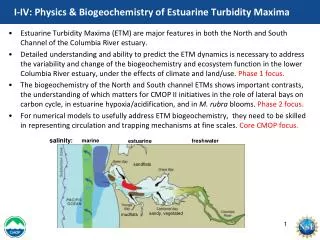
The dynamics of estuarine turbidity maxima. Stefan Talke * Huib de Swart * Victor de Jonge Groningen Workshop March 3, 2006. Overview. Experiments Analysis Modeling. Ultimate Goal: Understand the effect of biology and physical processes on each other and morphology.

E N D
The dynamics of estuarine turbidity maxima Stefan Talke * Huib de Swart * Victor de Jonge Groningen Workshop March 3, 2006
Overview • Experiments • Analysis • Modeling • Ultimate Goal: Understand the effect of biology and physical • processes on each other and morphology. • Preliminary Goal: Describe and analyze physical and • biological processes separately
Longitudinal Transects: 10 times since Feb. 2005 Cross-sectional Transects: Mar. 2005, Feb. 2006, Summer 2006? Overview of Experiments • Measurements at Longitudinal and Cross-Sectional Transects • Boats from RWS, WSA Emden, and NP GmBH used (Thanks!) • Both fixed station and continuous measurements Germany Netherlands
Water Fluid Mud Consolidated Bed • Measurements • ADCP (Acoustic Doppler Current Profiler) • Velocity measured continuously in water column (~0.5 Hz) • Backscatter used to estimate sediment concentration • Bottom tracking used to estimate boat velocity But, in turbid water, signal disappears! 600 kHz ADCP measures velocity and backscatter (turbidity) in 0.25 m increments
Water Fluid Mud Consolidated Bed • Measurements • Solution: • Use external echo-sounders and differential GPS Boat Velocity from GPS 210 kHz echosounder penetrates to the fluid mud layer
Measurements • Solution • Use external echo-sounders and differential GPS! Boat Velocity from GPS 15 kHz echosounder penetrates to the bed Water Fluid Mud Consolidated Bed
Measurements • On-board Flow-thru system Pump water into a bucket continuously Measure: Turbidity, Fluorescence, Salinity, Temperature, Oxygen Take care to prevent light, bubbles! Water Fluid Mud Consolidated Bed
Measurements • Fixed Point Measurements CTD Casts with OBS + Oxygen sensor measure Salinity, Temperature, Turbidity, Depth, Oxygen Water Samples (surface and water column) Analyzed for SSC, Organic Carbon, Nitrates, Silicates, Phosphorous, pH, Algal counts and types CTD Casts Water Samples Consolidated Bed
X X X X X X X X X • Measurements • Long Term Fixed Point Measurements: “X” • Monitored by NLWKN and WSA Emden • Measure: Tidal Stage, Salinity, Turbidity, Oxygen, pH, Velocity, Temperature, Sediment Concentration Germany CTD Casts Netherlands
Germany Longitudinal Transects Cross-sectional Transect: March 2005 Netherlands Cross-Sectional Data at Pogum
Fluid Mud 500 m Echosounder Data Transect at Pogum 8:27 am
Fluid Mud 500 m Echosounder Data Transect at Pogum 8:35 am
Fluid Mud 500 m Echosounder Data Transect at Pogum 9:21 am
Fluid Mud 500 m Echosounder Data Transect at Pogum 9:36 am
Fluid Mud 500 m Echosounder Data Transect at Pogum 10:03 am
Fluid Mud 500 m Echosounder Data Transect at Pogum 10:25 am
Fluid Mud 500 m Echosounder Data Transect at Pogum 10:36 am
Fluid Mud 500 m Echosounder Data Transect at Pogum 10:47 am
Fluid Mud 500 m Echosounder Data Transect at Pogum 11:22 am
Fluid Mud 500 m Echosounder Data Transect at Pogum 11:32 am
Fluid Mud 500 m Echosounder Data Transect at Pogum 15:11 pm
Fluid Mud 500 m Echosounder Data Transect at Pogum 15:14 pm
Fluid Mud 500 m Echosounder Data Transect at Pogum 15:56 pm
Fluid Mud 500 m Echosounder Data Transect at Pogum 16:00 pm Question: What does sediment concentration from ADCP backscatter look like?
Research Questions • What are the sediment concentrations • Analysis of ADCP data • What does mixing and turbulence look like over a tidal period • Research project of Robbert Schippers (Msc): • Analyze field data to estimate turbulent mixing • Apply GOTM 1-D vertical turbulence model
Sediment Calibration from Backscatter • Need to estimate attenuation of sound due to water and sediment Water attenuation (range 0.05-0.2)
Sediment Calibration from Backscatter • Highly dependant on grain size, density, frequency Sediment attenuation coefficient, 600 kHz Maximum at ~ 2 microns With 2 ADCP’s of differing frequency, can estimate mean grain size
Calculate Absolute backscatter • Loss is due to spreading of beam and attenuation • R= distance along beam to adcp bin (20 degrees offset from vertical) • E= measured backscatter • Alpha= combined, integrated attenuation • C,L,Kc,Er are instrument constants
Fit regression line sed-conc to abs. backscatter • Since attenuation depends on sediment concentration in profile… • make initial estimate of sed conc to calculate backscatter • Use backscatter to make linear regression • Re-estimate sediment concentration, recalculate attenuation, and repeat. • What about changes in floc size? • What about non-linear range? Non Linear Range Linear Range • Future Steps: • 1. Calibrate non-linear range with Feb. 2006 data • Estimate mean grain size using backscatter from 2 • ADCP’s on board one ship (Friesland)
Water level (m) Germany Netherlands Cross Section Sediment Concentration Profiles at Pogum (March 8,2005) Pogum
Water level (m) Time (hours) High turbidity evident Note structures in sediment profile mg/L Non-linear Range: > 5 g/L 8:30 am flood
Water level (m) Time (hours) Turbulence collapses, Sediment settles Sharp gradient between water and fluid mud Fluid mud pools in channel and shoal mg/L 11:30 am slack Non-linear Range: > 5 g/L
Water level (m) Time (hours) Very high turbidity and fluid mud mg/L Closer to ETM than earlier measurements 8:30 am Non-linear Range: > 5 g/L 16:00 Ebb
Vertical Observations: Interesting Salinity Profiles Flood (morning) Salinity often (but not always) decreases towards bed. Need to investigate density profiles…
Vertical Observations: Interesting Salinity Profiles Ebb (afternoon) As fluid mud is approached, salinity goes down. Measurment artifact? Or real physics? Why the low salinity? Perhaps not mixed with rest of water column? Are low salinities evidence of turbidity currents? How does mixing change between flood and ebb?
Vertical Observations—density profiles Including sediment concentration essential for water column stability Note again sharp transition to fluid mud
Vertical Observations—density gradients Positive means unstable Salinity profile dominates upper water column Sediment profile dominates lower water column
Vertical Observations—Richardson number 9:00 am (end of flood tide) • Richardson # measures • ratio of shear (turbulence) • to density gradient • (buoyancy) • >0.25 density dominates • < 0.25 shear dominates • < 0 Unstable Turbulence highly damped
Summary vertical and cross-section measurements • High sediment concentrations observed • How and at what tidal phase is sediment being mixed into upper water column? • Periodic formation of fluid mud layer • Collapse of turbulence, formation of flocs
Germany Longitudinal Transects—ADCP measurements in March, April, June, July, September 2005, and Feb. 2006 Netherlands Longitudinal Data
Longitudinal Results—Turbidity and Salinity Downstream Upstream From NP Aanderaa Probe In flow-through system Distance downstream from Herbrum (km) Large horizontal salinity and turbidity gradient (Turbidity not yet calibrated) Question: Are there density driven currents from both salinity and turbidity?
Longitudinal Results—Oxygen and Fluorescence Not yet calibrated—Fluorometer How are Dissolved oxygen and fluorescence related to the physical parameters of system?
Longitudinal Results--Salinity Knock Pogum Terborg Fixed NLWKN salinity measurements (note different scales)
Longitudinal Results--Sediment Knock Pogum Terborg Fixed NLWKN sediment concentration measurements Note concentrations of up to 10 g/L; in summer, > 25 g/L measured
Salinity gradient Combined gradient (salinity + sed. Conc.) Longitudinal Results—Density Gradients Knock-Pogum Pogum-Terborg Residual circulation proportional to density gradient Note that sediment density gradient changes sign
Thought Experiment • Consider “Bath Tub” Fresh Water (Salinity = 0) Circulation cell Heavy, turbid water flows along bottom Fresh water circulates to conserve mass Next, add turbid water to center What happens?
Thought Experiment • Consider another situation Salt Water (Ocean) Fresh Water (River) Now, consider case in which density differences occur only from salinity What Happens? Circulation cell from density difference due to salinity (gravitational circulation)
Salt Water Fresh Water Thought Experiment • Now, consider both together + Turbidity induced circulation Salinity induced circulation Hypothetical Combined Salt + turbidity circulatation = Salt Water Fresh Water
Thought Experiment Analysis: • Possible explanation for observed, asymmetric turbidity profiles? • To be realistic, need freshwater flow Q, bed slope, friction, etc. • Spread of turbid water critical for understanding depleted oxygen levels and other biological processes • Next step: Modeling Hypothetical Combined Salt + turbidity circulatation Salt Water Fresh Water Fresh Water
Development of Simple Model • We make the following assumptions: • No Tides—Consider only averages • Constant horizontal salinity gradient • Salinity well-mixed vertically • Sediment Concentration is prescribed • Balance between settling velocity and turbulent mixing