Download
1 / 20
200 likes | 507 Views
Constant Relative and Absolute Risk Aversion and Derivation of the State Contingent Dual Functions. Lecture XXXIV. Constant Relative and Absolute Risk Aversion. Risk Premium

E N D
Constant Relative and Absolute Risk Aversion and Derivation of the State Contingent Dual Functions Lecture XXXIV
Constant Relative and Absolute Risk Aversion • Risk Premium • Based on the definition of risk aversion from the preceding lecture, Chambers and Quiggin define the Risk Premium as the amount that a risk averse decision maker is willing to sacrifice to obtain a certain payoff.
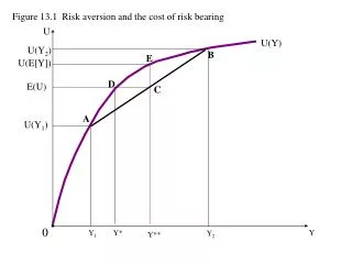
Fair-Odds Line 450
In this graph y is an outcome from a state-contingent output combination, however given risk aversion, the decision maker is indifferent between the state-contingent output combinationy* and y. Note that y* is a certain payoff because it is on the 450 line. • The certainty equivalent is the distance between point y and point y* in state-space.
Analytically, the absolute risk premium is defined by the benefit function:
The relative risk premium is then defined by the distance function:
Redefining constant absolute risk aversion • Definition 3.2 (p. 97): W displays constant absolute risk aversion if, for any y, for t R.
Fair-Odds Line 450
Redefining constant relative risk aversion • Definition 3.3 (p. 97): W displays constant relative risk aversion if, for any y, for t R.
Derivation of the Effort Function • From Lecture 33, we return to the notion of the valuation function as From this formulation, the valuation is dependent on the amount of effort applied (inputs used).
Properties of the Effort-Evaluation Function • gis nondecreasing and continuous for all x R. • g(x) = g(x) for all > 0, x R. • g(x + x0) g(x) + g(x0) x, x0 R.
Based on these properties Chambers and Quiggin define the effort-cost function as Note that this result states that the effort-cost function is defined as the minimum cost method of producing a given set of state contingent outputs.
Remember that X(z) is the set of all inputs that can be used to produce a vector of state contingent outputs, z.
If g(x) is a linear function, this relationship looks a lot like the standard cost-minimization model from duality. In fact, if the effort function is linear in input prices: where w is the vector of input prices. However, note that z is not a vector of deterministic outputs, but a vector of state-contingent outputs.
Shephard’s Lemma (p. 127):If a unique solution, x(w,z) R , exists to the minimization problem, the cost function is differentiable in w and
Putting it together (Chapter 5) • Under risk neutrality, the decision maker chooses the state-contingent outputs to maximize the expected return on production:
which can be transformed to Here C(w,r,p) is the revenue-cost function defined as
To demonstrate the implications of this model, consider the formulation under constant absolute riskiness. • First, Chambers and Quiggin define the certainty equivalent revenue as Defining the revenue vector as
Lemma 5.2 (p. 169): The technology displays constant absolute riskiness if and only if the revenue-cost function can be represented as where