Download
1 / 15
150 likes | 387 Views
Disaggregate State Level Freight Data to County Level. October 2013 Shih-Miao Chin, Ph.D. Ho-Ling Hwang, Ph.D. Francisco Moraes Oliveira Neto, Ph.D. Center for Transportation Analysis Oak Ridge National Laboratory. Outline. Background Freight Analysis Framework (FAF) Major data sources

E N D
Disaggregate State Level Freight Data to County Level October 2013 Shih-Miao Chin, Ph.D. Ho-Ling Hwang, Ph.D. Francisco Moraes Oliveira Neto, Ph.D. Center for Transportation Analysis Oak Ridge National Laboratory
Outline • Background • Freight Analysis Framework (FAF) • Major data sources • Methodology • Disaggregation process • Example • Results & Validations • FAF Ton-miles • Comparison with other freight data programs • Remarks
Eastern Asia Europe Africa South, Central & Western Asia Mexico Background: Freight Analysis Framework (FAF) • Manages by the Office of Freight Management and Operations, Federal Highway Administration (FHWA) • Provides a comprehensive picture of freight movement among states and major metropolitan areas by all modes • Most current release is FAF3.4 database Canada • Geography • 123 domestic regions • 8 foreign regions • Modes of transportation • Truck • Rail • Water • Air/air-truck • Multiple mode/mail • Pipeline • Others/unknown • 43 Commodities SW & Central Asia Eastern Asia SE Asia & Oceania Mexico Rest of Americas
Background: Major Data Sources • Commodity Flow Survey (CFS) • Conducted under the partnership of U.S. Census and Bureau of Transportation Statistics (BTS) • Sample survey of business U.S. establishments & classified according to North American Industry Classification System (NAICS) codes • Latest available data: 2007 (i.e., base year data for FAF3) • County Business Patterns (CBP) • An annual data series from U.S. Census • Provides economic data by industry (# establishments, employment, payroll) • Latest available data: 2011 • Industry Input-Output (I-O) Accounts • Annual I-O tables produced by the Bureau of Economic Analysis (BEA) • Make and Use Tables, by industry according to NAICS codes • Latest available data: 2011
FAF3 Disaggregation: Estimation of Ton-Miles • Tonnage and value of goods moved are important measures of the freight activity, but they do not necessarily reflect the usage of transportation systems • Environmental impact (emissions and fuel efficiency) of freight activity can be assessed using measures normalized by ton-miles • The revenue of transportation firms is related to the amount of freight in tones transported per mile • Main disaggregation steps • Linking freight activities with economic activities • Disaggregate FAF3 database (ODCM tonnage matrix) to county level • Estimate average shipment distance by mode on the multimodal network systems
Freight Flow Disaggregation Approach fFAFzone-to-zone, Commodity, Mode d o j i Attraction CBP BEA I-O Accounts (apq) Production CBP ωDestination county / Commodity, Mode ωOrigin county /Commodity, Mode Information theory ωcounty-to-county by commodity & mode ωO/C, M= ∑ωO / IωI / C, M ωD/C, M= ∑ωD / IωI / C, M Where (o, d) – FAF OD pair & (i, j) – County pair
Methodologies/Models • Log-linear regression models for linking freight activity with economic activity by industry sector at state • Production: freight tonnage shipped & payroll of producing industry • Attraction: freight tonnage received & payroll of receiving industry • Estimates of county-level production/attraction shares by industry • Spatial distribution by matrix balancing procedures (or doubly constraint gravity model)
Distance Matrices Intermodal Network Highway: Contains 500,000 miles of roadway in the US, Canada, and Mexico Railway: Contains every railroad route in the US, Canada, and Mexico that has been active since 1993 Waterway: Contains inland and off-shore links http://cta.ornl.gov/transnet/
Baltimore Example: 241 242 D = Estimated using the highway network system in GIS
FAF zone to county disaggregation – generation and attraction by county FAF O-D Flow (short tons) t242,241,truck = 171,747 Attraction Model (Attraction Share) Production Model (Production Share) Annual payroll ($ 1000) in the origin counties Share of annual payroll ($ 1000) in the destination counties
FAF to county disaggregation – distribution and spatial interaction
Matrix of Total Tons by Truck Matrix of Tons * Distance Matrix Matrix of Ton-miles
FAF Ton-miles Estimates Value/ Ton-miles ($) Include all domestic, exported, and imported shipments transported within the U.S.
Concluding Remarks • To carry out national transportation freight analysis and planning at a level of detail • The disaggregation methodology will provide more data at a more geographic detailed level for: • Environmental impact assessment • Vulnerability and resilience of freight multimodal network • Modal shift analysis • Truck weight and size studies • Further work is required to estimate freight flow models through FAF regions, by commodity, by mode.