Download

1 / 41
450 likes | 663 Views
Distributed Multipole Analysis. Ryan P. A. Bettens, Department of Chemistry, National University of Singapore. Intermolecular Interactions. High level ab initio calculations provide us with the most accurate means of determining intermolecular interactions.

E N D
Distributed Multipole Analysis Ryan P. A. Bettens, Department of Chemistry, National University of Singapore.
Intermolecular Interactions • High level ab initio calculations provide us with the most accurate means of determining intermolecular interactions. • Can only be applied to small systems, say a couple of dozen atoms. • Are extremely computationally expensive. • Are not feasible for use in simulations of the condensed phase. • Alternatively a perturbation approach can be used to evaluate the interaction energy. • Such an approach can explicitly consider the: • electrostatic interaction, • induction interaction, • dispersion interaction, • exchange repulsion.
The Electrostatic Interaction • Is entirely additive. • Evaluated by approximating YAB = yAyB where yA and yB are the ground state wavefunctions of molecules A and B respectively. • Such an approximation ignores electron exchange between molecules A and B, so steric repulsion is ignored. • Does not account for polarization nor dispersion in the first order interaction energy. • Turns: • Into:
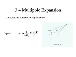
Central Multipoles • The are permanent multipoles placed at the origin of the molecule. • When l = 0, we have a monopole. • When l = 1, we have a dipole. • When l = 2, we have a quadrupole, etc. • Use of these central multipoles to compute the intermolecular electrostatic interaction suffers from significant convergence problems. • The multipole series diverges if the two molecules approach within the sum of their divergence sphere radii. • The divergence sphere is a sphere around a molecule that just encloses all the nuclei.
Distributed Multipoles • Convergence of the electrostatic interaction energy is greatly enhanced though the use if distributed multipoles. • Chemists are already familiar with distributed multipoles. • Consider H2O: • Treatment of the electrostatic interaction just with distributed monopoles, as we shall see, is very inaccurate. • We need to include higher order multipoles for greater accuracy. • How do we do this? d− ½d+ ½d+
Modeling the Electrostatic Potential Around Molecules • The electronic wavefunction of a molecule provides the electronic charge density in and around the nuclei. • By placing centers throughout the molecule the charge density can be analyzed in their vicinity. • The charge distribution about the centers give rise to multipoles at those centers, i.e., an overall charge at the center, a dipole, a quadrupole, etc. • These multipoles can then be used to predict the electrostatic potential at any location in space. • Let us consider how we can obtain these distributed multipoles from the electronic wavefunction.
Electronic Wavefunction • In ab initio calculations the electronic wavefunction is expanded in terms of the basis set employed. • A basis set is a collection of fixed mathematical gaussian functions (basis functions) with origins centered on each nuclei of the molecule. • Each molecular orbital is a linear combination of these basis functions (akin to LCAOMO). • The complete wavefunction is then written down as a Slater determinate (at the HF level) of the occupied molecular orbitals.
The Gaussian Functions • The gaussian functions that make up the basis set have the general form*: • The Rl,mare the regular spherical harmonics (l = 0, s-type orbital; l = 1, p-type orbital, etc.), and Nc is a normalization factor. • z is the exponent that dictates how close to the nucleus the electron is expected to be found. • A large z means the electron is held tight to the nucleus. • A small z means the electron can roam far from the nucleus. a r e− r − a
A Molecular Orbital • A molecular orbital is written as a linear combination of these basis functions: • Here the cs are the molecular orbital coefficients, which are determined in an ab initio calculation. • In GAUSSIAN these coefficients can be output by using the keywords “pop=full” in the route section.
H2O STO-3G Calculation Molecular Orbital Coefficients 1 2 3 4 5 (A1)--O (A1)--O (B2)--O (A1)--O (B1)--O EIGENVALUES -- -20.24288 -1.26659 -0.61482 -0.45348 -0.39127 1 1 O 1S 0.99414 -0.23293 0.00000 -0.10321 0.00000 2 2S 0.02646 0.83508 0.00000 0.53668 0.00000 3 2PX 0.00000 0.00000 0.00000 0.00000 1.00000 4 2PY 0.00000 0.00000 0.60690 0.00000 0.00000 5 2PZ -0.00432 -0.12846 0.00000 0.77438 0.00000 6 2 H 1S -0.00592 0.15833 0.44555 -0.28013 0.00000 7 3 H 1S -0.00592 0.15833 -0.44555 -0.28013 0.00000 6 7 (A1)--V (B2)--V EIGENVALUES -- 0.60190 0.73572 1 1 O 1S -0.13155 0.00000 2 2S 0.87580 0.00000 3 2PX 0.00000 0.00000 4 2PY 0.00000 0.98672 5 2PZ -0.74440 0.00000 6 2 H 1S -0.79336 -0.83485 7 3 H 1S -0.79336 0.83485
The Density Matrix • The density matrix, P, can be directly obtained from the molecular orbital coefficients. • For a HF calculation the density matrix is just: • Here cs,i is the molecular orbital coefficient for basis function s and molecular orbital i. • The summation is taken over the occupied molecular orbitals only. • For doubly occupied orbitals each product is multiplied by 2, as there are two electrons in each molecular orbital.
Density Matrix for H2O STO-3G • PO1s,O2s = 2(0.99414 × 0.02646 + −0.23293 × 0.83508 + 0.00000 × 0.00000 + −0.10321 × 0.53668 + 0.00000 × 0.00000) = −0.44720 DENSITY MATRIX. 1 2 3 4 5 1 1 O 1S 2.10645 2 2S -0.44720 1.97216 3 2PX 0.00000 0.00000 2.00000 4 2PY 0.00000 0.00000 0.00000 0.73664 5 2PZ -0.10859 0.61640 0.00000 0.00000 1.23238 6 2 H 1S -0.02770 -0.03656 0.00000 0.54081 -0.47449 7 3 H 1S -0.02770 -0.03656 0.00000 -0.54081 -0.47449 6 7 6 2 H 1S 0.60419 7 3 H 1S -0.18987 0.60419
Charge Density • The density matrix is utilized in finding the charge density at some (x,y,z) = r point in space. • That is • Note that this charge density can also include the effects of electron correlation, which can be incorporated into P. • Note that the charge density at some point r depends on products of the gaussian basis functions.
Charge Density and Multipoles • We now have a formula for the charge density at any point is space. • A multipole can be directly determined from this charge density via • However, this multipole is a central multipole, or a multipole for the entire molecule. • We wish to determine a set of distributed multipoles. • We have to ensure not to “double count” the charge density in computing the multipoles at different sites. • We need to take a closer look at our expression for the charge density to see how we might assign density to different sites.
Product of Gaussian Basis Functions • Consider the product csct • It can be shown that the product of two gaussians centered at different origins, here at and as, is a single gaussian at a new origin ptslying somewhere on the line joining the two origins, which are nuclei. • That is where Just a constant
E.g. of Gaussian Overlap First gaussian (G1) with z = 1. Second gaussian (G2) with z = 0.25. Overlap gaussian / 0.049, with z = 1.25.
Shifting the regular Spherical Harmonics • The product of two basis functions also contains the regular spherical harmonics, Rl,m and Rl’,m’. • Each of these spherical harmonics can be shifted to the new origin that the gaussian is about, i.e., shifted to point pst. • The shift can be obtained from the spherical harmonic addition theorem. • The two terms in the square-root are binomial coefficients. Just a constant
Shifting Both the Regular Spherical Harmonics to the Same Origin • The previous expression shows that shifting the regular spherical harmonic Rl,mto a new origin produces a linear combination of regular spherical harmonics from rank 0 to rank l. • The same can be done for Rl’,m’, so that for this regular spherical harmonic we also obtain a linear combination of regular spherical harmonics up to rank l’.
Basis Function Product – a function now about a single origin • We have arrived at an expression for the product of two basis functions • which occurs in our formula for the charge density, • that originally involved functions centered on different origins, i.e., sites as and at, • but now is a linear combination of functions with a common origin, pst. • Unfortunately this linear combination of functions still involves products of the type.
Products of Regular Spherical Harmonics • The product of two regular spherical harmonic located at the same origin is a linear combination of regular spherical harmonics that range in rank from |l−l’| to l+l’. • Thus the final product of two basis functions, csct, is a rather complicated linear combination of terms of the form: • which involve regular spherical harmonics of ranks 0 to l+l’.
The Charge Density • We can now write the electronic part of the charge density as • The term in the charge density has multipole moments, evaluated with origin at pst, that are all zero except for Qk,q. • Hence the product of basis functions csct, with angular momentum l and l’ has multipole moments, with respect to origin pst, of ranks from 0 to l+l’ only.
Multipoles Arising from the Charge Density • An exact multipole representation of the charge distribution consists of a set of multipoles for each product of primitive gaussians appearing in the charge density. • Because the number of basis functions can be large, up to thousands, then the number of these products can be up to millions – this seems not particularly convenient. • Still, most basis sets employed do not extend to particularly large values of l. • Often only s, p and d type functions are used, i.e., l = 0, l = 1 and l = 2 respectively.
Basis Function Overlap • Overlap of two s-type functions gives rise to a point charge only (l + l’ = 0) centered at pst. • Overlap of an s-type with a p-type will give rise to a charge and dipole centered at pst. • Overlap of two p-type functions will give rise to a charge, dipole and quadrupole centered at pst. • Etc. Charge distribution from this product pst Tight s-function More diffuse s-function A point charge at pst exactly* represents the potential from this product distribution.
Distributing the Multipoles. • Although exact, it is not convenient to have lots and lots of little multipole expansions about all the possible pst’s. • We need to shift these multipoles back onto the atomic centers, or whatever sites we have chosen for our distributed multipole approach. • This is where some degree of arbitrariness arises. • The decision of how to divide the multipoles up onto nearby sites is know as the allocation algorithm.
Shifting a Multipole • To shift a multipole from some point to another requires us to employ again the spherical harmonic addition theorem. • Again, the regular spherical harmonics are the definition of the multipole moment operators, so we can immediately write down the expression for a new multipole moment at origin c in terms of the original multipoles.
Shifting a Multipole • Even if the charge distribution is described exactly in terms of a finite number of multipole moments, there will be multipole moments up to rank infinity if a different origin is chosen. • Consider, for example Na+. • One and only one multipole describes the charge distribution of this atom, i.e., Q0,0 = 1, all other moments vanish. • If we now wish to shift the origin to (0,0,c) then we have the following non-zero moments: Q0,0 = 1, Q1,0 = −c, Q2,0 = c2, Q3,0 = −c3, Q4,0 = c4,… • If the origin shift is too far then these moments rapidly become very large.
Divergence Sphere Reduced • A divergence sphere no longer exists for the entire molecule, but now for each site. • The divergence sphere for a distributed multipole site is centered at the site origin and must be just large enough to enclose all multipoles that are to be transferred to it. • Depending on the allocation algorithm this may reduce the divergence sphere compared to the central multipole expansion considerably.
The Mulliken Allocation Algorithm • Is trivially simple. • 50% of the multipole at pst is assigned to site s and 50% is assigned to site t from whence the basis functions came. • Simplicity is the only advantage of the Mulliken allocation algorithm. • The disadvantage of the Mulliken allocation algorithm is that it may involve large shifts of the multipoles, especially if the sites are far apart.
The Mulliken Allocation Algorithm • If one of the exponents is much larger than the other, then the overlap center, pst, may be very close to one of the sites. • Regardless of this fact, the Mulliken allocation algorithm will shift 50% of the multipoles onto the far site. • This relatively large shift also has an impact on the divergence sphere. • E.g., two atoms are several bonds apart, but diffuse basis functions are employed. There may be significant overlap between a diffuse function and a regular basis function on the other atom. In this case: • The divergence sphere must reach across several bond lengths. • 50% of the multipoles must be shifted across several bond lengths.
Mulliken Charges and Distributed Monopoles • These charges are obtained by: • Using the Mulliken allocation algorithm. • Ignoring multipoles at psthigher than Q0,0. • It should be very clear at this point that such an approximation to the electrostatic potential of a molecule is: • wildly inaccurate and • not particularly convergent. • In fact any distributed charge model using atomic sites clearly suffers for the complete neglect of the multipoles with l ≥ 1 that arise at pstdue to overlap of any basis functions other than a pair of s-type functions. • Worse, even using only the Q0,0 at pstshifting this charge to different origins requires higher multipole moments at the new origins to retain the accuracy.
Graphically Representing the Mulliken Allocation Algorithm • Regardless of how far pstis from both sites, 50% of the charge is shifted to both sites. • This separation of charge generates a dipole field, if pst is not exactly ½ way between the sites, when none is present. • In order to accurately represent the point charge at pst with multipoles at sites s and t, dipoles and higher multipoles are also needed at sites s and t. pst A point charge at pst exactly* represents the potential from this product distribution. Charge distribution from this product 50% of the charge is shifted to site s 50% of the charge is shifted to site t Tight s-function More diffuse s-function
The Nearest-Site Allocation Algorithm • Allocate all of the multipoles to the nearest site. • As simple as the Mulliken allocation algorithm, but considerably more convergent and requires fewer multipoles due to shorter multipole shifts. • The divergence sphere is never larger than ½ the distance to the nearest site. • This algorithm has been shown to be considerably more accurate than the Mulliken algorithm. • Was the original algorithm implemented by Stone in his earlier work, and is obtained now using GDMA with the “switch=0.0” card.
The Nearest-Site Allocation Algorithm • One disadvantage of the nearest-site allocation algorithm is that the distributed multipoles are sensitive to basis set employed. • This occurs because a change of basis involves changes in the exponents, z, so the overlap centers, pst, are different for different basis sets. • The allocation of a particular set of overlap multipoles to one site or another depends on whether the corresponding pstfalls to one side or the other of the dividing surface between the sites. • Thus small changes in the positions of the overlap centers can have dramatic effects on the multipole moments. • Note that this is not so much an issue for the interaction energy.
Illustration of the Problem with the Nearest-Site Allocation Algorithm • Consider CO2 in a large and diffuse basis. • There may be a diffuse primitive pz on C. • There may be a diffuse primitive s on each O (labeled A and B). • The linear combination √½(sA− sB) will be very similar to pzC. • The densities associated with these two functions are: (pzC)2 and ½(sA− sB)2 = ½(sA)2 − sAsB + ½(sB)2 • The multipoles associated with the (pzC)2 density is centered on C and are Q0,0 = −1 and Q2,0 (Q1,0 = 0). • The multipoles associated with the ½(sA− sB)2 are centered on the two O atoms (si)2 and the C atom sAsB (C is the nearest site to pAB). • The multipoles are −½q on each O atom and +q − 1 on the C atom. • A basis set change will have different exponents and might easily lead to a difference in the preference of one or the other of these.
Improved Allocation Algorithm • The issue with the nearest-site algorithm is that the allocation is performed in basis-set space, rather than the more sensible physical space. • Numerical integration (quadrature) over physical space can be performed. • A grid of integration points is constructed about each atom. • The molecular grid is the union of the atom grids. • Every point in space has associated with it a set of atom weights. • The sum of the weights for any point is 1. • The nearest atom to the point has a weight close to 1, and other atoms near 0 weight.
Improved Allocation Algorithm • At the boundary between two atoms the weight of one atom falls smoothly to 0 as the weight of the other increases to 1. • Achieved by a “smoothing” function. • Density is partitioned thus into overlapping regions, each assigned to one atom. • Here rela(r) is the density partitioned to atom a. • The multipoles are then obtained by numerical integration.
Comparing Old and New Allocation Algorithms • If the sum of the exponents in the overlap is greater than 4.0, then the nearest-site algorithm is used. • Compare the nearest-site algorithm to the new algorithm.
Comparing Old and New Allocation Algorithms • The differences between the old (switch = 0) and new (switch = 4) methods in the electrostatic potential on the vdW× 2 surface are still less than 1% of the potential itself.
Central, Mulliken, DMA versus ab Initio Electrostatic Potentials Point +1 charge approaching O along C2 axis in H2O. Central Multipole
CHARMM, Mulliken, NPA, DMA versus ab Initio Electrostatic Potentials Solvent accessible surface