Download

1 / 21
210 likes | 358 Views
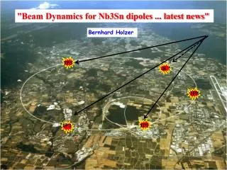
”Beam Dynamics for Nb3Sn dipoles ... latest news". Bernhard Holzer. IP5. IR 7. IP8. IP1. IP2. *. DS Upgrade Scenarios. halo. Shift 12 Cryo -magnets, DFB, and connection cryostat in each DS. transversely shifted by 4.5 cm. halo. New ~3..3.5 m shorter Nb 3 Sn Dipoles (2 per DS).

E N D
”Beam Dynamics for Nb3Sn dipoles ... latest news" Bernhard Holzer IP5 IR 7 IP8 IP1 IP2 *
DS Upgrade Scenarios halo Shift 12 Cryo-magnets, DFB, and connection cryostat in each DS transversely shifted by 4.5 cm halo New ~3..3.5 m shorter Nb3Sn Dipoles (2 per DS) -4.5m shifted in s +4.5 m shifted in s M. Karppinen TE-MSC-ML
Effects to be expected: * magnets are shorter than MB Standards change of geometry distortion of design orbit * R-Bends S-Bends edge focusing distortion of the optics tune shift, beta beat * nonlinar transfer function (3.5 TeV) distortion of closed orbit to be corrected locally ?? dedicated corrector coils ?? trim power supply ?? * feed down effects from sagitta ? * multipole effect on dynamic aperture ? Sixtrack Tracking Simulations
The persistent current problem: Very First Multipole Estimates tracking studies & prototype measurements needed b3 remanence as a function of precycle (pre-injection plateau) B.Auchmann Comparison: b3 Hysteresis Nb3Sn / NbTi M. Karppinen
Nb3Sn Dipole: Multipole Errors, “Pure Estimation !!” ... in the usual units, i.e. 10 -4 referred to the usual ref radius = 17mm
Where are we ? IP1,2,5,IP7 Q8 Q9 Q10 Present Option: 2 x 5.5m Nb3Sn Dipoles separated
optics situation collision optics, 7 TeV no big difference in optical functions between injection / luminosity
Tracking Studies: Dynamic Aperture determined via stability / survival time theory: phase space ellipse defined by optical parameters ideal, linear machine strong b3 multipole Phase Space Distance b3 = 98, full & local correction b3 = 98, no correction
Tracking Studies: Dynamic Aperture determined via survival time b3 = 98, no correction survival time ... measured in number of turns ... gives an indication of the influence of the non-linear fields on the ( an- ) harmonic oscillation of the particles. y For the experts: 60 seeds, 10^5 turns, 4-18 σ in units of 2, 30 particle pairs, 17 angles x
Field Quality: Dynamic Aperture Studies 7 TeV Case, luminosity optics (55cm) ε=5*10-10 radm ( εn= 3.75μm) ideal Nb3Sn dipoles mult. coeff. à la error table6 at high field the higher harmonics are small enough, the p.c. effects disappeared and the emittance is reduced (Liouville)
Field Quality: Dynamic Aperture Studies injection optics, 450 GeV, influence of b3 values, 2 IP’s = 8 dipoles dyn aperture injection optics, minimum of 60 seeds dynamic aperture for Nb3Sn full error table (blue) b3 = 0 an = bn = 0 the first estimated errors lead to extreme reduction in dyn. aperture main problem: b3
Field Quality: Dynamic Aperture Studies Injection Optics, 450 GeV, Scan of b3 dyn aperture injection optics, minimum of 60 seeds dynamic aperture for Nb3Sn case: full error table (red) b3 reduced to 50% (green) b3 reduced to 25% (violett) b3 = 0 and to compare with: present LHC injection for the experts: unlike to the collision case: at injection the b3 of the Nb3Sn dipoles is the driving force to the limit in dynamic aperture. A scan in b3 values has been performed and shows that values up to b3 ≈ 20 units are ok.
Field Quality: Dynamic Aperture Studies Injection Optics, 450 GeV, Different Sectors dyn aperture for Nb3Sn dipoles in #2,7 and in #1,2,5 standard spool piece correctors optimised for Q’ correction per octant #2,7, an=bn=0 #2,7 b3=27 #1,2,5 b3=27 #2,7 first estimate, “error table 2”
Field Quality: Dynamic Aperture Studies Injection Optics, 450 GeV, ATS dyn aperture for Nb3Sn dipoles #1,2,5 ATS shows a increased sensitivity for higher multipoles, -> tighter limit for b3 and higher an / bn ATS Lattice #1,2,5 an=bn=0 #1,2,5 b3=0 #1,2,5 bn=20 #1,2,5 b3=27
Field Quality: Dynamic Aperture Studies Injection Optics, 450 GeV, first measured values: “FNAL-demo-2” measured values for the “systematics” FNAL best guess for the ramndom errors Mikko et al
Field Quality: Dynamic Aperture Studies Injection Optics, 450 GeV, first measured values: “FNAL-demo-2” and again the tracking ... systematics -> FNAL prototype random -> best guess uncertainty - > MB standard dipole ideal Nb3Sn dipoles, an=bn=0 first FNAL prototype systematics & Mikkos random artificially enhanced b4...6 , a3 first measured values are just at the limit but at the moment in sufficient dynamic aperture is obtained.
Preliminary (!) Resumée: first estimates / calculations for pc systematics ... where chilling limits calculated for higher multipole coefficients (mainly b3) first measurement results are “just within” these limits problem: injection energy / optics large emittance, large p.c. effects ATS injection / luminosity seems a bit more sensitive than LHC standard optics unknown: realistic values for random errors ? do we have to deal with uncertainties ? limits for individual higher coefficients Plan & Next Steps: follow up closely the new results
ParticleTrackingCalculations particlevector: field at particleposition Idea: calculatetheparticlecoordiantes x, x´ throughthe linear lattice … usingthematrixformalism. ifyouencounter a nonlinearelement (e.g. sextupole): stop calculateexplicitlythemagneticfield at theparticlescoordinate calculate kick on the particle and continue with the linear matrix transformations