Download
1 / 49
490 likes | 598 Views
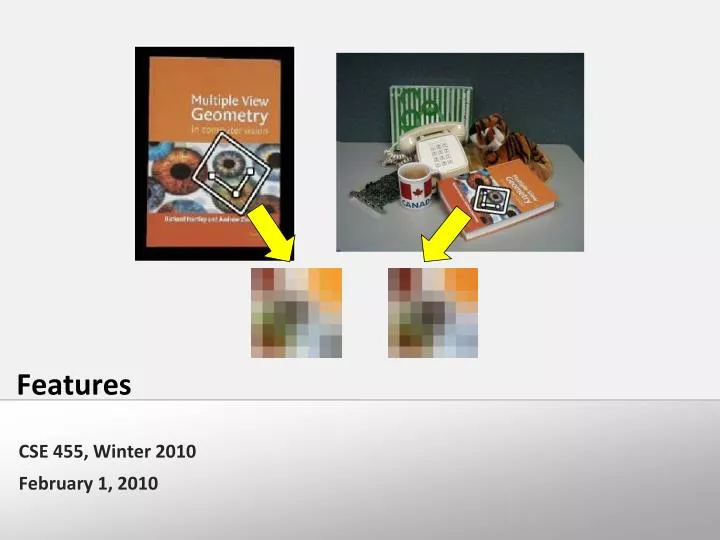
Features. CSE 455, Winter 2010 February 1 , 2010. Review From Last Time. Measuring height. 5.4. 5. Camera height. 4. 3.3. 3. 2.8. 2. 1. The cross ratio. A Projective Invariant Something that does not change under projective transformations (including perspective projection).

E N D
Features CSE 455, Winter 2010 February 1, 2010
Measuring height 5.4 5 Camera height 4 3.3 3 2.8 2 1
The cross ratio • A Projective Invariant • Something that does not change under projective transformations (including perspective projection) The cross-ratio of 4 collinear points P4 P3 P2 P1 • Can permute the point ordering • 4! = 24 different orders (but only 6 distinct values) • This is the fundamental invariant of projective geometry
Monocular Depth Cues • Stationary Cues: • Perspective • Relative size • Familiar size • Aerial perspective • Occlusion • Peripheral vision • Texture gradient
Camera calibration • Goal: estimate the camera parameters • Version 1: solve for projection matrix • Version 2: solve for camera parameters separately • intrinsics (focal length, principle point, pixel size) • extrinsics (rotation angles, translation) • radial distortion
Calibration using a reference object • Place a known object in the scene • identify correspondence between image and scene • compute mapping from scene to image • Issues • must know geometry very accurately • must know 3D->2D correspondence
Alternative: multi-plane calibration Images courtesy Jean-Yves Bouguet, Intel Corp. • Advantage • Only requires a plane • Don’t have to know positions/orientations • Good code available online! • Intel’s OpenCV library:http://www.intel.com/research/mrl/research/opencv/ • Matlab version by Jean-Yves Bouget: http://www.vision.caltech.edu/bouguetj/calib_doc/index.html • Zhengyou Zhang’s web site: http://research.microsoft.com/~zhang/Calib/
Today • Features • What are Features? • Edges • Corners • Generally “interesting” parts of an image All is Vanity, by C. Allan Gilbert, 1873-1929 • Readings • M. Brown et al. Multi-Image Matching using Multi-Scale Oriented Patches, CVPR 2005
Edge detection • Convert a 2D image into a set of curves • Extracts salient features of the scene • More compact than pixels
Image gradient • The gradient of an image: The gradient points in the direction of most rapid increase in intensity • The gradient direction is given by: • how does this relate to the direction of the edge? • The edge strength is given by the gradient magnitude
The Canny edge detector • original image (Lena)
The Canny edge detector norm of the gradient
The Canny edge detector thresholding
The Canny edge detector thinning (non-maximum suppression)
Image matching by Diva Sian by swashford TexPoint fonts used in EMF. Read the TexPoint manual before you delete this box.: AAAAAA
Harder case by Diva Sian by scgbt
Even harder case “How the Afghan Girl was Identified by Her Iris Patterns” Read the story
Harder still? NASA Mars Rover images
Answer below (look for tiny colored squares…) NASA Mars Rover images with SIFT feature matchesFigure by Noah Snavely
Invariant local features • Find features that are invariant to transformations • geometric invariance: translation, rotation, scale • photometric invariance: brightness, exposure, … Feature Descriptors
Advantages of local features • Locality • features are local, so robust to occlusion and clutter • Distinctiveness: • can differentiate a large database of objects • Quantity • hundreds or thousands in a single image • Efficiency • real-time performance achievable • Generality • exploit different types of features in different situations
More motivation… • Feature points are used for: • Image alignment (e.g., mosaics) • 3D reconstruction • Motion tracking • Object recognition • Indexing and database retrieval • Robot navigation • … other
What makes a good feature? Snoop demo
Want uniqueness • Look for image regions that are unusual • Lead to unambiguous matches in other images • How to define “unusual”?
Local measures of uniqueness • Suppose we only consider a small window of pixels • What defines whether a feature is a good or bad candidate? Slide adapted form Darya Frolova, Denis Simakov, Weizmann Institute.
Feature detection • Local measure of feature uniqueness • How does the window change when you shift it? • Shifting the window in any direction causes a big change “corner”:significant change in all directions “flat” region:no change in all directions “edge”: no change along the edge direction Slide adapted form Darya Frolova, Denis Simakov, Weizmann Institute.
Feature detection: the math • Consider shifting the window W by (u,v) • how do the pixels in W change? • compare each pixel before and after bysumming up the squared differences (SSD) • this defines an SSD “error” of E(u,v): W
Small motion assumption • Taylor Series expansion of I: • If the motion (u,v) is small, then first order approx is good • Plugging this into the formula on the previous slide…
Feature detection: the math • Consider shifting the window W by (u,v) • how do the pixels in W change? • compare each pixel before and after bysumming up the squared differences • this defines an “error” of E(u,v): W
Feature detection: the math This can be rewritten: • For the example above • You can move the center of the green window to anywhere on the blue unit circle • Which directions will result in the largest and smallest E values? • We can find these directions by looking at the eigenvectors ofH
Quick eigenvalue/eigenvector review • The eigenvectors of a matrix A are the vectors x that satisfy: • The scalar is the eigenvalue corresponding to x • The eigenvalues are found by solving: • In our case, A = H is a 2x2 matrix, so we have • The solution: • Once you know , you find x by solving
Feature detection: the math This can be rewritten: x- x+ • Eigenvalues and eigenvectors of H • Define shifts with the smallest and largest change (E value) • x+ = direction of largest increase in E. • + = amount of increase in direction x+ • x- = direction of smallest increase in E. • - = amount of increase in direction x+
Feature detection: the math • How are +, x+, -,and x+ relevant for feature detection? • What’s our feature scoring function?
Feature detection: the math • How are +, x+, -,and x+ relevant for feature detection? • What’s our feature scoring function? • Want E(u,v) to be large for small shifts in all directions • the minimum of E(u,v) should be large, over all unit vectors [u v] • this minimum is given by the smaller eigenvalue (-) of H
Feature detection summary • Here’s what you do • Compute the gradient at each point in the image • Create the H matrix from the entries in the gradient • Compute the eigenvalues. • Find points with large response (-> threshold) • Choose those points where - is a local maximum as features
Feature detection summary • Here’s what you do • Compute the gradient at each point in the image • Create the H matrix from the entries in the gradient • Compute the eigenvalues. • Find points with large response (-> threshold) • Choose those points where - is a local maximum as features
The Harris operator • - is a variant of the “Harris operator” for feature detection • The trace is the sum of the diagonals, i.e., trace(H) = h11 + h22 • Very similar to - but less expensive (no square root) • Called the “Harris Corner Detector” or “Harris Operator” • Lots of other detectors, this is one of the most popular
The Harris operator Harris operator