Download
1 / 11
110 likes | 313 Views
The cycle of a Genetic Algorithms is presented below. Each cycle in Genetic Algorithms produces a new generation of possible solutions for a given problem. Genetic Algorithm Steps. The elements of the population are encoded into bit-strings , called chromosomes.

E N D
The cycle of a Genetic Algorithms is presented below Each cycle in Genetic Algorithms produces a new generation of possible solutions for a given problem
Genetic Algorithm Steps • The elements of the population are encoded into bit-strings, called chromosomes. • The performance of the strings, often called fitness, is then evaluated with the help of some functions f(x) , representing the constraints of the problem. • The crossover operation that recombines the bits (genes) of each two selected strings (chromosomes) . The crossover helps to span over the solution space
Genetic Algorithm Steps In Mutation the bits at one or more randomly selected positions of the chromosomes are altered. The mutation process helps to overcome trapping at local maxima Mutation of a chromosome at the 5th bit position. Example: The Genetic Algorithms cycle is illustrated in this example for maximizing a function f(x) = x2in the interval 0 = x = 31. In this example the fitness function is f (x) itself. Starts with 4 initial strings. The fitness value of the strings and the percentage fitness of the total are estimated in Table A.
Example Table A • Since fitness of the second string is large, we select 2 copies of the second string and one each for the first and fourth string in the mating pool. The selection of the partners in the mating pool is also done randomly • Here in table B, we selected partner of string 1 to be the 2-nd string and partner of 4-th string to be the 2nd string. The crossover points for the first-second and second-fourth strings have been selected after 0-th and 2-nd bit positions respectively in table B. Table B
Example 1 -\IEEE_OPTIM_2012\GA\gaex.m The second generation of the population without mutation in the first generation is presented in table C. Table C >> gatool %- Solution % gaex.m function f=gaex(x) f=-x*x; %Maximize >> load gaexoptim >> gaexoptions
Example 1- \IEEE_OPTIM\_2012\GA \gaex.m 0-4 => 5 bits 25 =32 => [0;31] Fitness f(x) x -variable
Example 2 -\IEEE_OPTIM_2012\GA\Live_fn_gatool.m Example 2 %Live_fn_gatool.m % >>Load optimproblem.mat %Start >>GATOOL % Import from workspace 'optimproblem' function fposition=Live_fn_gatool(x) fposition=(x(1)+1.42513)^2+(x(2)+.80032)^2; 1. Use Gatool and maximize the quadratic equation f(x) = x2 +4x-1 within the range −5 ≤x≤0. 2. Use Gatool and maximize the function f(x1, x2, x3)= −5 sin(x1) sin(x2) sin(x3) + (- sin(5x1) sin(5x2)sin(x3)) where 0 <= xi <= pi, for 1 <= i <= 3. 3. Create a “gatool” to minimize the function f(x) = cos(2x) within the range 0≤x≤3.14
Eample 3 - Genetic Algorithm with Simulink \IEEE_OPTIM_2012\GA\motor_select_opt_ga.m %lead_screw_model_opt_Motor_ga.mdl %motor_select_ga_fun.m %load gaoptions.mat clc Ki=0.1, Ka=1; u0=[Ki,Ka]; options=gaoptimset(options,'PopulationSize',10,'TimeLimit',100, 'Generations',200,'StallTimeLimit',20,'TolCon',1e-6,'TolFun',1e-6) [x,funct]=ga(@motor_select_ga_fun,2,[],[],[],[],[0.001 0.001],[],[],options) function funct=motor_select_ga_fun(x) Ki=x(1); Ka=x(2); assignin('base','Ki', Ki); assignin('base','Ka', Ka); [t, xout, err]=sim('lead_screw_model_opt_Motor_ga',[0 10]); funct=sqrt(sum(err).^2);
Example 4 \IEEE_OPTIM\_2012\GA \Live_fn_ga.m hold off clf clc [y, fposition]=ga(@Live_fn_ga, 2); x=y fposition; %3-D plot. [X,Y]=meshgrid(-5:0.1:5,-5:0.1:5); Z=(X+1.42513).^2+(Y+.80032).^2; surf(X,Y,Z), hold plot(y(1),y(2),'or') function fposition=Live_fn_ga(x) t=1; u=[x(1),x(2)]; dt=t; [t, xout, y]=sim('Live_fn_simGA',t,simset('MaxDatapoints',1),[t,u]); fposition=y;