Download
1 / 21
210 likes | 425 Views
Nearest-neighbor matching to feature database. Hypotheses are generated by matching each feature to nearest neighbor vectors in database No fast method exists for always finding 128-element vector to nearest neighbor in a large database Therefore, use approximate nearest neighbor:

E N D
Nearest-neighbor matching to feature database • Hypotheses are generated by matching each feature to nearest neighbor vectors in database • No fast method exists for always finding 128-element vector to nearest neighbor in a large database • Therefore, use approximate nearest neighbor: • We use best-bin-first (Beis & Lowe, 97) modification to k-d tree algorithm • Use heap data structure to identify bins in order by their distance from query point • Result: Can give speedup by factor of 1000 while finding nearest neighbor (of interest) 95% of the time
Detecting 0.1% inliers among 99.9% outliers • Need to recognize clusters of just 3 consistent features among 3000 feature match hypotheses • LMS or RANSAC would be hopeless! • Use generalized Hough transform • Vote for each potential match according to model ID and pose • Insert into multiple bins to allow for error in similarity approximation • Using a hash table instead of an array avoids need to form empty bins or predict array size
Probability of correct match • Compare distance of nearest neighbor to second nearest neighbor (from different object) • Threshold of 0.8 provides excellent separation
Model verification • Examine all clusters in Hough transform with at least 3 features • Perform least-squares affine fit to model. • Discard outliers and perform top-down check for additional features. • Evaluate probability that match is correct • Use Bayesian model, with probability that features would arise by chance if object was not present • Takes account of object size in image, textured regions, model feature count in database, accuracy of fit (Lowe, CVPR 01)
Solution for affine parameters • Affine transform of [x,y] to [u,v]: • Rewrite to solve for transform parameters:
Models for planar surfaces with SIFT keys Planar texture models
Planar recognition • Planar surfaces can be reliably recognized at a rotation of 60° away from the camera • Affine fit approximates perspective projection • Only 3 points are needed for recognition
3D Object Recognition • Extract outlines with background subtraction
3D Object Recognition • Only 3 keys are needed for recognition, so extra keys provide robustness • Affine model is no longer as accurate
Test of illumination invariance • Same image under differing illumination 273 keys verified in final match
Robot Localization • Joint work with Stephen Se, Jim Little
Recognizing Panoramas • Matthew Brown and David Lowe • Recognize overlap from an unordered set of images and automatically stitch together • SIFT features provide initial feature matching • Image blending at multiple scales hides the seams Panorama of our lab automatically assembled from 143 images
Comparison to template matching • Costs of template matching • 250,000 locations x 30 orientations x 4 scales = 30,000,000 evaluations • Does not easily handle partial occlusion and other variation without large increase in template numbers • Viola & Jones cascade must start again for each qualitatively different template • Costs of local feature approach • 3000 evaluations (reduction by factor of 10,000) • Features are more invariant to illumination, 3D rotation, and object variation • Use of many small subtemplates increases robustness to partial occlusion and other variations