Download
1 / 37
380 likes | 441 Views
Department of Mathematics Maheshtala College. Systems of Linear Equations. Presented by Ajijur Rahaman Mallick. Contents. 1.1 Introduction to Systems of Linear Equations 1.2 Gaussian Elimination and Gauss-Jordan Elimination. 1.1 Introduction to Systems of Linear Equations.

E N D
Department of Mathematics Maheshtala College Systems of Linear Equations Presented by Ajijur Rahaman Mallick
Contents • 1.1 Introduction to Systems of Linear Equations • 1.2 Gaussian Elimination and Gauss-Jordan Elimination
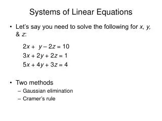
1.1Introduction to Systems of Linear Equations • a linear equation in n variables: a1,a2,a3,…,an, b: real number a1: leading coefficient x1: leading variable • Notes: (1) Linear equations have no products or roots of variables and no variables involved in trigonometric, exponential, or logarithmic functions. (2) Variables appear only to the first power.
such that • a solution of a linear equation in n variables: • Solution set: the set of all solutions of a linear equation
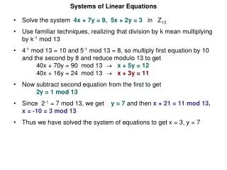
If you solve for x1 in terms of x2, you obtain By letting you can represent the solution set as And the solutions are or • Ex 2: (Parametric representation of a solution set) a solution: (2, 1), i.e.
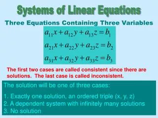
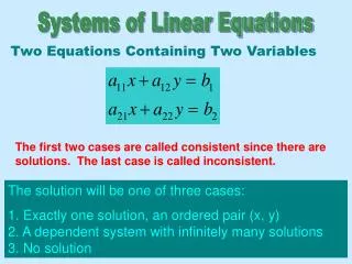
a system of m linear equations in n variables: • Consistent: A system of linear equations has at least one solution. • Inconsistent: A system of linear equations has no solution.
Notes: Every system of linear equations has either (1) exactly one solution, (2) infinitely many solutions, or (3) no solution.
Ex 4: (Solution of a system of linear equations) (1) (2) (3)
Sol: By substituting into (1), you obtain The system has exactly one solution: • Ex 5: (Using back substitution to solve a system in row echelon form)
Sol: Substitute into (2) and substitute and into (1) The system has exactly one solution: • Ex 6: (Using back substitution to solve a system in row echelon form)
Equivalent: Two systems of linear equations are called equivalent if they have precisely the same solution set. • Notes: Each of the following operations on a system of linear equations produces an equivalent system. (1) Interchange two equations. (2) Multiply an equation by a nonzero constant. (3) Add a multiple of an equation to another equation.
Sol: • Ex 7: Solve a system of linear equations (consistent system)
So the solution is (only one solution)
Sol: • Ex 8: Solve a system of linear equations (inconsistent system)
Sol: • Ex 9: Solve a system of linear equations (infinitely many solutions)
let then So this system has infinitely many solutions.
(3) If , then the matrix is called square of order n. 1.2 Gaussian Elimination and Gauss-Jordan Elimination • mn matrix: • Notes: (1) Every entry aij in a matrix is a number. (2) A matrix with m rows and n columns is said to be of size mn . (4) For a square matrix, the entries a11, a22, …, ann are called the main diagonal entries.
Ex 1: Matrix Size • Note: One very common use of matrices is to represent a system of linear equations.
Matrix form: • a system of m equations in n variables:
Coefficient matrix: • Augmented matrix:
Elementary row operation: (1) Interchange two rows. (2) Multiply a row by a nonzero constant. (3) Add a multiple of a row to another row. • Row equivalent: Two matrices are said to be row equivalent if one can be obtained from the other by a finite sequence of elementary row operation.
Ex 3: Using elementary row operations to solve a system Linear System Associated Augemented Matrix Elementary Row Operation
Elementary Row Operation Associated Augemented Matrix Linear System
Row-echelon form: (1, 2, 3) • Reduced row-echelon form: (1, 2, 3, 4) (1) All row consisting entirely of zeros occur at the bottom of the matrix. (2) For each row that does not consist entirely of zeros, the first nonzero entry is 1 (called a leading 1). (3) For two successive (nonzero) rows, the leading 1 in the higher row is farther to the left than the leading 1 in the lower row. (4) Every column that has a leading 1 has zeros in every position above and below its leading 1.
Gaussian elimination: The procedure for reducing a matrix to a row-echelon form. • Gauss-Jordan elimination: The procedure for reducing a matrix to a reduced row-echelon form. • Notes: (1) Every matrix has an unique reduced row echelon form. (2) A row-echelon form of a given matrix is not unique. (Different sequences of row operations can produce different row-echelon forms.)
Produce leading 1 The first nonzero column Produce leading 1 leading 1 The first nonzero column Submatrix Zeros elements below leading 1 • Ex: (Procedure of Gaussian elimination and Gauss-Jordan elimination)
leading 1 Submatrix Zeros elements below leading 1 Produce leading 1 Zeros elsewhere leading 1
Sol: • Ex 7: Solve a system by Gauss-Jordan elimination method (only one solution)
Sol: • Ex 8:Solve a system by Gauss-Jordan elimination method (infinitely many solutions)
Let So this system has infinitely many solutions.
Homogeneous systems of linear equations: A system of linear equations is said to be homogeneous if all the constant terms are zero.
Trivial solution: • Nontrivial solution: other solutions • Notes: (1) Every homogeneous system of linear equations is consistent. (2) If the homogenous system has fewer equations than variables, then it must have an infinite number of solutions. (3) For a homogeneous system, exactly one of the following is true. (a) The system has only the trivial solution. (b) The system has infinitely many nontrivial solutions in addition to the trivial solution.
Let Sol: • Ex 9: Solve the following homogeneous system