Download
1 / 35
350 likes | 505 Views
Indicators and Scenarios. Today. The objectives of SUTRA SUTRA and the DPSIR framework The set of indicators The set of scenarios The methodology for the economic assessment. The objectives of SUTRA. Model-based elaborations of scenarios of urban development

E N D
Today • The objectives of SUTRA • SUTRA and the DPSIR framework • The set of indicators • The set of scenarios • The methodology for the economic assessment
The objectives of SUTRA • Model-based elaborations of scenarios of urban development • using transport, emission, air quality, energy system analysis, health and economic assessment modules • Set of indicators used for baseline analysis, ranking and benchmarking
Questions • How to define the set of indicators? • How to define the set of scenarios?
Demography Land-use Economy Technology direct and Economic indirect costs of . Assess transportation Exposition to noise Consumption of fossil fuels Stress indicators Demand Markal time loss for congestion (OD matrix) TREM Visum Emissions Emissions Ofis Concentrations Public Vadis ESS (O3 ) Health Morbidity, Concentrations mortality (CO et al) (pollution and
The set of indicators • Consistent with the DPSIR framework and the current literature • Summarising all the information contained in the input and output of all models • traffic, emission, air quality, energy system analysis, health, economic assessment used in SUTRA
The set of indicators • Driving forces • Economic, demographic, land-use variables • Pressures • Transport demand and emissions (CO2, NOx, VOC, CO, PM10) • State • Air quality (concentration of pollutants), noise and stress indicators (jams, overcrowded public transports) • Impacts • Mortality and morbidity, direct and external costs • Responses • Car occupancy, public vs. private transport, market penetration of new technologies (EV, HEV, FCEV)
The set of indicators • Driving forces • Economic, demographic, land-use variables • Pressures • Transport demand and emissions (CO2, NOx, VOC, CO, PM10) • State • Air quality (concentration of pollutants), noise and stress indicators (jams, overcrowded public transports) • Impacts • Mortality and morbidity, direct and external costs • Responses • Car occupancy, public vs. private transport, market penetration of new technologies (EV, HEV, FCEV)
The set of indicators • Driving forces • Economic, demographic, land-use variables • Pressures • Transport demand and emissions (CO2, NOx, VOC, CO, PM10) • State • Air quality (concentration of pollutants), noise and stress indicators (jams, overcrowded public transports) • Impacts • Mortality and morbidity, direct and external costs • Responses • Car occupancy, public vs. private transport, market penetration of new technologies (EV, HEV, FCEV)
The set of indicators • Driving forces • Economic, demographic, land-use variables • Pressures • Transport demand and emissions (CO2, NOx, VOC, CO, PM10) • State • Air quality (concentration of pollutants), noise and stress indicators (jams, overcrowded public transports) • Impacts • Mortality and morbidity, direct and external costs • Responses • Car occupancy, public vs. private transport, market penetration of new technologies (EV, HEV, FCEV)
The set of indicators • Driving forces • Economic, demographic, land-use variables • Pressures • Transport demand and emissions (CO2, NOx, VOC, CO, PM10) • State • Air quality (concentration of pollutants), noise and stress indicators (jams, overcrowded public transports) • Impacts • Mortality and morbidity, direct and external costs • Responses • Car occupancy, public vs. private transport, market penetration of new technologies (EV, HEV, FCEV)
The set of indicators • Driving forces • Economic, demographic, land-use variables • Pressures • Transport demand and emissions • State • Air quality (concentration of pollutants), noise and stress indicators • Impacts • Mortality and morbidity, direct and external costs • Responses • Car occupancy, public vs. private transport, market penetration of new technologies (EV, HEV, FCEV)
Scenarios • Changes in a set of external driving forces and policy decisions • Translation into model input variables and parameters
Defining future urban scenarios: 4 big issues • Demographic changes • Economic structure changes • Technological changes • Land-use changes • Each issue is defined by a set of parameters which vary within a interval of sensible values
Demographic scenarios • Two issues • Demographic urban growth and decline • The ageing of urban population
Urban growth and decline 1.5 1 Stockholm Oslo Helsinki Strasbourg Utrecht Malmoe Thessaloniki Amsterdam Wien Hamburg 0.5 Paris London Rotterdam Population growth over 1990-98 Napoli Kopenavhn Madrid Antwerpen Lazio Milano Bremen Lille Barcelona 0 Birmingham Athina Bruxelles Liverpool Genova Bilbao -0.5 Lisboa -1 -1 -0.5 0 0.5 1 1.5 Population growth over 1980-89 74% 156% Source: Camb. Econometrics
Urban ageing Source: UNDP
Economic scenarios • Three issues • Economic growth • Shift towards services • Increasing use of telework
Towards a 100% service economy Source: Camb. Econometrics
Increasing teleworking? • Home based-teleworkers • one full day per week • Occasional teleworkers • less than one full day per week • In Europe (ECaTT, % of total labour force) • 1999. 6.1% teleworkers, 2% home-based • 2005. 10.8% teleworkers, 4.2% home-based • High variety of situations • Finland home-based, from 6.7% to 16.7% • Spain home-based from 1.3% to 2.7%
Land use scenarios • Two issues • Urban sprawl • densification of less-developed areas and expansion at the urban fringe • EEA, 1999, speaks of “increasing dispersal and sprawling of urban settlements with declining urban population densities and greater requirements for urban infrastructure” • Mixing urban functions • locates land uses with complementary functions close together
Technological scenarios • Four issues • Passenger car occupancy rate • Modal share: public and private transport • Information Technology in traffic control & management • Penetration rates of new technologies
Technologies: towards a more efficient use of cleaner technologies? • Traffic control • Alternative fuels: Electric Vehicles, Hybrid Electric Vehicles, Fuel Cell Electric Vehicles
Technologies: towards a more efficient use of cleaner technologies? Average urban occupancy rate in 10 European cities from 1990 to 2000 Source: Auto Oil II
Technologies: towards a more efficient use of cleaner technologies? Average modal shares in 10 European cities from 1990 to 2000 Source: Auto Oil II
Summary of scenarios ISSUES ADDRESSED Baseline Upper end Lower end Demographic changes The city is growing and The city is shrinking and getting younger getting older Economic structural The city is changing fast The city is changing slowly changes towards a high-tech service- towards a high-tech service- based economy based economy Technological changes The city is moving fast The city is moving slowly Current situation towards improving transport towards improving transport efficiency efficiency Land-use changes The city is densifying and The city is sprawling and mixing land uses separating land uses
Summary of scenarios BASELINE UPPER END LOWER END SCENARIOS CURRENT STATE DEMOGRAPHIC Average EU cities growth GROWTH - 1 % pa GROWTH + 1.5 % CHANGES 1980-2000 [74% pop2000] [156% pop2000] population size 0.4% pa DEMOGRAPHIC Expected changes 2000-2030 CHANGES (UNPD) YOUTH –5pp YOUTH 0pp WA – 10pp WA – 3pp population age YH – 2pp, WA –5pp, OAP +8pp OAP +15pp OAP +3pp Average EU cities changes 1980-2000 ECONOMIC SERVICES + 5pp SERVICES + 20pp SERVICES+ 11pp CHANGES TELEW = 15% TELEW = 70% Teleworkers MIN 2.8% (Spain) MAX 16.8% (Finland) City areas increases City areas decreases EU cities Three circles of urban functions Proportional distribution of urban LAND USE Increasing dispersal and sprawling of CHANGES urban settlements function
Selection of common scenarios • Dynamic, rich and virtuous city • a young and growing city moving fast to high-tech services jobs, which cares about the environment and adopts clean technologies and careful planning • Dynamic, rich and vicious city • a young and growing city moving fast to high-tech services jobs, which, however, saves on clean technologies and grow chaotically into the countryside around • Virtuous pensioners city • a city becoming a city of pensioners, it does not grow, does not change its economic structures, yet, it cares about the environment and adopts clean technologies and careful planning • Vicious pensioner city • a city becoming a city of pensioners, it does not grow, does not change its economic structures. It does not adopt clean technologies or careful planning
Demography Land-use Economy Technology direct and Economic indirect costs of . Assess transportation Exposition to noise Consumption of fossil fuels Stress indicators Demand Markal time loss for congestion (OD matrix) TREM Visum Emissions Emissions Ofis Concentrations Public Vadis ESS (O3 ) Health Morbidity, Concentrations mortality (CO et al) (pollution and
Economic assessment Environment Climate change Full cost External costs Human health Crops Buildings Noise Landscape Congestion Accidents Use of space Infrastructure costs Direct costs Private costs Fuel Maintenance Repairs Insurance tax Cost of vehicle Time Source: Quinet (1997)
Direct and external costs (per capita) 4,00 Young virtuous 3,50 3,00 Young vicious 2,50 External costs (Baseline=1) 2,00 Old virtuous 1,50 1,00 Old vicious 0,50 0,00 0,00 0,50 1,00 1,50 2,00 2,50 Genova 4 Genova 2 Genova 1 Genova 3 Direct costs (Baseline=1)
Direct and external costs Young virtuous Old virtuous Genova Lisboa Gdansk Young vicious Old vicious Thessaloniki Tel Aviv Genève
Direct and external costs (per pkm) 3,00 Genova 4 Young virtuous city 2,50 Genova 2 2,00 Young vicious city Genova 1 External costs (Baseline=1) 1,50 Old virtuous 1,00 Genova 3 0,50 Old vicious 0,00 0,00 0,50 1,00 1,50 2,00 2,50 Direct costs (Baseline=1)