Download
1 / 29
290 likes | 393 Views
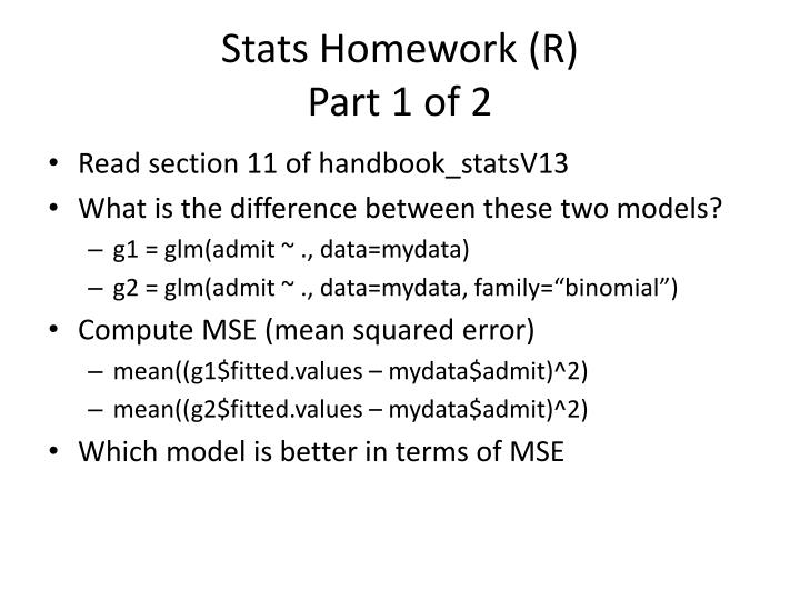
Stats Homework (R ) Part 1 of 2. Read section 11 of handbook_statsV13 What is the difference between these two models? g1 = glm(admit ~ ., data= mydata ) g2 = glm(admit ~ ., data= mydata , family=“binomial”) Compute MSE (mean squared error) mean((g1$fitted.values – mydata$admit)^2)

E N D
Stats Homework (R)Part 1 of 2 • Read section 11 of handbook_statsV13 • What is the difference between these two models? • g1 = glm(admit ~ ., data=mydata) • g2 = glm(admit ~ ., data=mydata, family=“binomial”) • Compute MSE (mean squared error) • mean((g1$fitted.values – mydata$admit)^2) • mean((g2$fitted.values – mydata$admit)^2) • Which model is better in terms of MSE
Stats Homework (R)Part 2 of 2 • Consider two loss functions • MSE.loss = function(y, yhat) mean((y - yhat)^2) • log.loss= function(y, yhat) -mean(y * log(yhat) + (1-y) * log(1-yhat)) • Which model (g1 or g2) is better in terms of loss2? • Hint:log.lossassumesyhatis a probability between 0 and 1 • What are range(g1$fitted.values) and range(g2$fitted.values)? • Let s = g1$fitted.values > 0 & g1$fitted.values < 1 • What islog.loss(mydata$admit[s], g1$fitted.values[s])? • Let baseline.fit be rep(mean(admit), length(admit)) • How do the two models above compare to this baseline • Compare both g1 and g2 to this baseline using both loss functions
Functions • fact = function(x) if(x < 2) 1 else x*fact(x-1) • fact(5) • fact2 = function(x) gamma(x+1) • fact(5) • fact(1:5) • fact(seq(1,5,0.5))
What are statistics packages good for? • Plotting • Scatter plots, histograms, boxplots • Visualization • Dendrograms, heatmaps • Modeling • Linear Regression • Logistic Regression • Hypothesis Testing
Objects Data Types Operations All: summary, help, print, cat Numbers: +,*,sqrt Strings: grep, substr, paste Vectors: x = (3:30) x+5 plot(x) mean(x), var(x), median(x) mean((x – mean(x))^2) x[3], x[3:6], x[-1], x[x>20] Matrices: m = matrix(1:100,ncol=10) m+3, m* 3, m %*% m m[3,3], m[1:3,1:3], m[3,], m[m < 10] diag(m), t(m) Data Frames names(swiss) plot(swiss$Education, swiss$Fertility) plot(swiss[,1], swiss[,2]) pairs(swiss) • Numbers: 1, 1.5 • Strings • Functions: • sqrt, help, summary • Vectors: • 3:30 • c(1:5, 25:30) • rnorm(100, 0, 1), rbinom(100, 10, .5) • rep(0,10) • scan( filename, 0) • Matrices • matrix(rep(0,100), ncol=10) • diag(rep(1,10)) • cbind(1:10, 21:30) • rbind(1:10, 21:30) • Data Frames • swiss • read.table (filename, header=T)
plot(swiss$Education, swiss$Fertility, col = 3 + (swiss$Catholic > 50))
boxplot(split(swiss$Fertility, swiss$Education > median(swiss$Education)))
Correlations > cor(swiss$Fertility, swiss$Catholic) [1] 0.4636847 > cor(swiss$Fertility, swiss$Education) [1] -0.6637889 > round(100*cor(swiss)) Fertility Agriculture Examination Education Catholic Infant.Mortality Fertility 100 35 -65 -66 46 42 Agriculture 35 100 -69 -64 40 -6 Examination -65 -69 100 70 -57 -11 Education -66 -64 70 100 -15 -10 Catholic 46 40 -57 -15 100 18 Infant.Mortality 42 -6 -11 -10 18 100 • Many functions in R are polymorphic: • cor works on vectors as well as matrices
Regression > plot(swiss$Education, swiss$Fertility) > g = glm(swiss$Fertility ~ swiss$Education) > abline(g) > summary(g) Call: glm(formula = swiss$Fertility ~ swiss$Education) Deviance Residuals: Min 1Q Median 3Q Max -17.036 -6.711 -1.011 9.526 19.689 Coefficients: Estimate Std. Error t value Pr(>|t|) (Intercept) 79.6101 2.1041 37.836 < 2e-16 *** swiss$Education -0.8624 0.1448 -5.954 3.66e-07 *** --- Signif. codes: 0 ‘***’ 0.001 ‘**’ 0.01 ‘*’ 0.05 ‘.’ 0.1 ‘ ’ 1 (Dispersion parameter for gaussian family taken to be 89.22746) Null deviance: 7178.0 on 46 degrees of freedom Residual deviance: 4015.2 on 45 degrees of freedom AIC: 348.42 Number of Fisher Scoring iterations: 2
plot(swiss$Education, swiss$Fertility, type='n’); abline(g)text(swiss$Education, swiss$Fertility, dimnames(swiss)[[1]])
g = glm(Fertility ~ . , data=swiss); summary(g) Call: glm(formula = Fertility ~ ., data = swiss) Deviance Residuals: Min 1Q Median 3Q Max -15.2743 -5.2617 0.5032 4.1198 15.3213 Coefficients: Estimate Std. Error t value Pr(>|t|) (Intercept) 66.91518 10.70604 6.250 1.91e-07 *** Agriculture -0.17211 0.07030 -2.448 0.01873 * Examination -0.25801 0.25388 -1.016 0.31546 Education -0.87094 0.18303 -4.758 2.43e-05 *** Catholic 0.10412 0.03526 2.953 0.00519 ** Infant.Mortality 1.07705 0.38172 2.822 0.00734 ** --- Signif. codes: 0 ‘***’ 0.001 ‘**’ 0.01 ‘*’ 0.05 ‘.’ 0.1 ‘ ’ 1 (Dispersion parameter for gaussian family taken to be 51.34251) Null deviance: 7178.0 on 46 degrees of freedom Residual deviance: 2105.0 on 41 degrees of freedom AIC: 326.07 Number of Fisher Scoring iterations: 2
http://www.nytimes.com/2009/01/07/technology/business-computing/07program.htmlhttp://www.nytimes.com/2009/01/07/technology/business-computing/07program.html
Plot Example • help(ldeaths) • plot(mdeaths, col="blue", ylab="Deaths", sub="Male (blue), Female (pink)", ylim=range(c(mdeaths, fdeaths))) • lines(fdeaths, lwd=3, col="pink") • abline(v=1970:1980, lty=3) • abline(h=seq(0,3000,1000), lty=3, col="red")
Periodicity • plot(1:length(fdeaths), fdeaths, type='l') • lines((1:length(fdeaths))+12, fdeaths, lty=3)
Type Argument par(mfrow=c(2,2)) plot(fdeaths, type='p', main="points") plot(fdeaths, type='l', main="lines") plot(fdeaths, type='b', main="b") plot(fdeaths, type='o', main="o")
ScatterPlot • plot(as.vector(mdeaths), as.vector(fdeaths)) • g=glm(fdeaths ~ mdeaths) • abline(g) • g$coef (Intercept) mdeaths -45.2598005 0.4050554
Hist & Density • par(mfrow=c(2,1)) • hist(fdeaths/mdeaths, nclass=30) • plot(density(fdeaths/mdeaths))
Data Frames • help(cars) • names(cars) • summary(cars) • plot(cars) • cars2 = cars • cars2$speed2 = cars$speed^2 • cars2$speed3 = cars$speed^3 • summary(cars2) • names(cars2) • plot(cars2) • options(digits=2) • cor(cars2)
Normality par(mfrow=c(2,1)) plot(density(cars$dist/cars$speed)) lines(density(rnorm(1000000, mean(cars$dist/cars$speed), sqrt(var(cars$dist/ cars$speed)))), col="red") qqnorm(cars$dist/cars$speed) abline(mean(cars$dist/cars$speed), sqrt(var(cars$dist/cars$speed)))
Stopping Distance Increases Quickly With Speed • plot(cars$speed, cars$dist/cars$speed) • boxplot(split(cars$dist/cars$speed, round(cars$speed/10)*10))
Quadratic Model of Stopping Distance plot(cars$speed, cars$dist) cars$speed2 = cars$speed^2 g2 = glm(cars$dist ~ cars$speed2) lines(cars$speed, g2$fitted.values)
Bowed Residuals g1 = glm(dist ~ poly(speed, 1), data=cars) g2 = glm(dist ~ poly(speed, 2), data=cars) par(mfrow=c(1,2)) boxplot(split(g1$resid, round(cars$speed/5))); abline(h=0) boxplot(split(g2$resid, round(cars$speed/5))); abline(h=0)
Help, Demo, Example • demo(graphics) • example(plot) • example(lines) • help(cars) • help(WWWusage) • example(abline) • example(text) • example(par) • boxplots • example(boxplot) • help(chickwts) • demo(plotmath) • pairs • example(pairs) • help(quakes) • help(airquality) • help(attitude) • Anorexia • utils::data(anorexia, package="MASS") • pairs(anorexia, col=c("red", "green", "blue")[anorexia$Treat]) • counting • example(table) • example(quantile) • example(hist) • help(faithful)
Randomness • example(rnorm) • example(rbinom) • example(rt) • Normality • example(qqnorm) • Regression • help(cars) • example(glm) • demo(lm.glm)