Earthquake Location

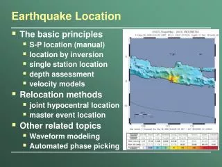
Earthquake Location by Annabel Kelly

Overview • The basic principles • S-P location (manual) • location by inversion • single station location • depth assessment • velocity models • Relocation methods • joint hypocentral location • master event location • Other related topics • Waveform modeling • Automated phase picking USGS

Basic Principles • 4 unknowns - origin time, x, y, z • Data from seismograms – phase arrival times March 28, 2005 M8.7 Sumatra earthquake, as recorded at GNI station in Armenia (60 Degrees from the epicenter)

S-P time • Time between P and S arrivals increases with distance from the focus. • A single trace can therefore give the origin time and distance (but not azimuth) approximates to PREM model, Dziewonski & Anderson, 1981

Courtesy of Dr. Qamar-uz-Zaman Chaudhary Pakistan Mteorological Dept.

S-P method • 1 station – know the distance - a circle of possible location • 2 stations – two circles that will intersect at two locations • 3 stations – 3 circles, one intersection = unique location 4+ stations – over determined problem – can get an estimation of errors Source: Japan Meteorological Agency

Wadati diagram S-P time against absolute P arrival time • gives the origin time (where S-TP time = 0) • Determines Vp/Vs (assuming it’s constant and the P and S phases are the same type – e.g. Pn and Sn, or Pg and Sg) • indicates pick errors

Locating with P only • The location has 4 unknowns (t,x,y,z) so with 4+ P arrivals this can be solved. • The P arrival time has a non-linear relationship to the location, even in the simplest case when we assume constant velocity – therefore can only be solved numerically

ti= √(x0-xi)2+(y0-yi)2 v Numerical methods • Calculated travel time: • Simplest possible relation between travel time and location: • Find location by minimizing the summed residual (e): tci= T(xi,yi,zi,x0,y0,z0) + t0 n ri= ti– tci e = Σ(ri)2 i=1

Least squares – the outlier problem • The squaring makes the solution very sensitive to outliers. • Algorithms normally leave out points with large residuals

Numerical methods – grid search courtesy of Robert Mereu

starting location calc solution true location residual 1 2 3 4 iteration solving using linearization • It’s possible to solve directly using math: • Assume a starting location • Assume that the change needed is small enough that is can be considered a linear change • Counteract the approximation of linearizing the problem by taking the solution as a new starting model.

The residuals are not always a well behaved function, can have local minima A grid search may show if there is a better solution courtesy of Robert Mereu

Single station method Particle motion – P wave N • The S-P time give the distance to the epicenter • The ratio of movement on the horizontal components gives the azimuth Station W E to event S UP UP Station N W E to event W March 28, 2005 M8.7 Sumatra earthquake, as recorded at ARU station in Russia (62 Degrees from the epicenter) DOWN

Depth estimation ANSS station spacing ~280 km • The distance between the station and the event is likely to be many kilometers. Therefore a small variation in focal depth (e.g. 5 km) will have little effect on the distance between the event and the station. • Therefore the S-P time and P arrival time are insensitive to focal depth tens to hundreds of kilometers 10 km 20 km

Synthetic tests of variation in depth resolution - used in designing the network. • As the distance for the quake to the nearest station increases the network becomes insensitive to the depth of the event (which was 10km for this test data). courtesy of Robert Mereu

Depth – pP and sP • The phases that reflect from the Earth surface near the course (pP and sP) can be used to get a more accurate depth estimate Stein and Wysession “An Introduction to Seismology, Earthquakes, and Earth Structure”

Velocity models • For distant events may use a 1-D reference model (e.g. PREM) and station corrections PREM model, Dziewonski & Anderson, 1981

Local velocity model • For local earthquakes need a model that represents the (1D) structure of the local crust. SeisGram2K

Determining the local velocity model • Refraction data the best for Moho depth and velocity structure of the crust. Annabel Kelly

Art Jolly http://www.giseis.alaska.edu/Seis/Input/martin/physics212/seismictomo.html Tomography • Local tomography from local earthquakes can give crust and upper mantle velocities • Regional/Global tomography from global events gives mantle velocity structure. Seismic Tomography at the Tonga Arc Zone (Zhao et al., 1994)

Station Corrections • Station corrections allow for local structure and differences from the 1D model Contours of the P-wave Station Correction, NE India Courtesy J R Kayal (Bhattacharya et al., 2005)

Good location Poor location Location in subduction zones • Poor station distribution

Operational Planned Courtesy L. Kong Stations in the Indian Ocean

Network locations relocations Relocation methods • Recalculate the locations using the relationship between the events. • Master Event Method • Joint hypocentral determination • Double difference method Waldhauser and Schaff “Improving Earthquake Locations in Northern California Using Waveform Based Differential Time Measurements”

Master event relocation • Select master event(s) – quakes with good locations, probably either the largest magnitude or event(s) that occurred after a temporary deployment of seismographs. • Assign residuals from this event as the station corrections. • Relocated other events using these station corrections.

Joint Hypocenter Determination (JHD) • In JHD a number of events are located simultaneously solving for the station correction that minimizes the misfit for all events. (rather than picking one “master event” that is assumed to have good locations).

Difference in calculated arrival time for stations i and j Double difference for event k – aim to minimize this residual Difference in observed arrival time for stations i and j Double difference method • This approach doesn’t calculate station corrections. • Instead the relative position of pairs of events is adjusted to minimize the difference between the observed and calculated travel time differences

Analyst Picks Cross-correlated Picks Cross-correlation to improve picks • Phases from events with similar locations and focal mechanisms will have similar waveforms. • realign traces to maximize the cross-correlation of the waveform. Rowe et al 2002. Pure and Applied Geophysics 159

Simultaneous inversion • Calculate the velocity structure and relocate the earthquakes at the same time. • Needs very good coverage of ray paths through the model. Model for Parkfield California – 15 stations, 6 explosions, 453 earthquakes Thurber et al. 2003. Geophysical Research Letters

Some additional related topics... • Waveform modeling • Automated phase pickers • location of great earthquakes

Waveform modeling • Generate synthetic waveforms and compare to the recorded data to constrain the event  Stein and Wysession “An Introduction to Seismology, Earthquakes, and Earth Structure”

Waveform modeling Construction of the synthetic seismogram u(t) = x(t) * e(t) * q(t) * i(t) U(ω)= X(ω) E(ω) Q(ω) I(ω) source time function attenuation instrument response reflections & conversions at interfaces seismogram

Automatic phase picks • Short term average - long term average (STA/LTA) – developed in the 1970s, still used by Earthworm and Sac2000 Sleeman and von Eck 1999, Physics of Earth and Planetary Interiors 113

Autoregression analysis • Autoregression (AR) models the seismogram as predictable signal + noise • Find the point at which predictable signal can be identified using Akaike Information Criterion (AIC) from the AR of series in the noise and in the phase. Leonard and Kennett 1999, Physics of Earth and Planetary Interiors 113

CUSUM algorithm • Looks for a change in the cumulative sum of a statistic that defines a change in properties. • Calculate a CUSUM of a statistic and subtract the trend (converts changes in the trend to minima) look for minima in this function Where Ck is the cumulative squared amplitude (up to point K) and CT is the sum of x2 over the whole window of T points) Der and Shumway 1999, Physics of Earth and Planetary Interiors 113

Location of Great Earthquakes • With great earthquakes the slip area is very large (hundreds of kilometers) • For hazard assessment the epicenter and centroid are not very informative. Need to rupture area, but this is not available in time for tsunami warnings/disaster management. Epicenter Centroid Lay et al 2006, Science 308

Earthquake Location