Download
1 / 18
180 likes | 306 Views
Bayes for Beginners Rumana Chowdhury & Peter Smittenaar Methods for Dummies 2011 Dec 7 th 2011. A disease occurs in 0.5% of population A diagnostic test gives a positive result in 99% of people that have the disease in 5% of people that do not have the disease (false positive)

E N D
Bayes for Beginners RumanaChowdhury & Peter Smittenaar Methods for Dummies 2011 Dec 7th 2011
A disease occurs in 0.5% of population • A diagnostic test gives a positive result • in 99% of people that have the disease • in 5% of people that do not have the disease (false positive) A random person from the street is found to be positive on this test. What is the probability that they have the disease? A: 0-30% B: 30-60% C: 60-90%
A disease occurs in 0.5% of population • A diagnostic test gives a positive result • in 99% of people that have the disease • in 5% of people that do not have the disease (false positive) A = disease B = positive test result P(A) = 0.005 probability of having disease P(~A) = 1 – 0.005 = 0.995 probability of not having disease P(B) = 0.005 * 0.99 (people with disease) + 0.995 * 0.05 (people without disease) = 0.0547 (slightly more than 5% of all tests are positive) conditional probabilities P(B|A) = 0.99 probability of pos result given you have disease P(~B|A) = 1 – 0.99 = 0.01 probability of neg result given you have disease P(B|~A) = 0.05 probability of pos result given you do not have disease P(~B|~A) = 1 – 0.05 = 0.95 probability of neg result given you do not have disease P(A|B) is probability of disease given the test is positive (which is what we’re interested in) Very different from P(B|A): probability of positive test results given you have the disease.
A = disease B = positive test result population = 100 positive test result P(B) 5.47 disease P(A) 0.5
population = 100 A = disease B = positive test result P(A,B) is the joint probability, or the probability that both events occur. P(A,B) is the same as P(B,A). But we already know that the test was positive, so we have to take that into account. Of all the people already in the green circle, how many fall into the P(A,B) part? That’s the probability we want to know! That is: P(A|B) = P(A,B) / P(B) You can write down same thing for the inverse: P(B|A) = P(A,B) / P(A) The joint probability can be expressed in two ways by rewriting the equations P(A,B) = P(A|B) * P(B) P(A,B) = P(B|A) * P(A) Equating the two gives P(A|B) * P(B) = P(B|A) * P(A) P(A|B) = P(B|A) * P(A) / P(B) positive test result P(B) 5.47 P(B,~A) disease P(A) 0.5 P(A,B) P(A,~B)
A = disease B = positive test result P(A) = 0.005 probability of having disease P(B|A) = 0.99 probability of pos result given you have disease P(B) = 0.005 * 0.99 (people with disease) + 0.995 * 0.05 (people without disease) = 0.0547 Bayes’ Theorem P(A|B) = P(B|A) * P(A) / P(B) P(A|B) = 0.99 * 0.005 / 0.0547 = 0.09 So a positive test result increases your probability of having the disease to ‘only’ 9%, simply because the disease is very rare (relative to the false positive rate). P(A) is called the prior: before we have any information, we estimate the chance of having the disease 0.5% P(B|A) is called the likelihood: probability of the data (pos test result) given an underlying cause (disease) P(B) is the marginal probability of the data: the probability of observing this particular outcome, taken over all possible values of A (disease and no disease) P(A|B) is the posteriorprobability: it is a combination of what you thought before obtaining the data, and the new information the data provided (combination of prior and likelihood)
Let’s do another one… It rains on 20% of days. When it rains, it was forecasted 80% of the time When it doesn’t rain, it was erroneously forecasted 10% of the time. The weatherman forecasts rain. What’s the probability of it actually raining? • A = forecast rain • B = it rains • What information is given in the story? • P(B) = 0.2 (prior) • P(A|B) = 0.8 (likelihood) • P(A|~B) = 0.1 • P(B|A) = P(A|B) * P(B) / P(A) • What is P(A), probability of rain forecast? Calculate over all possible values of B (marginal probability) • P(A|B) * P(B) + P(A|~B) * P(~B) = 0.8 * 0.2 + 0.1 * 0.8 = 0.24 • P(B|A) = 0.8 * 0.2 / 0.24 • = 0.67 • So before you knew anything you thought P(rain) was 0.2. Now that you heard the weather forecast, you adjust your expectation upwards P(rain|forecast) = 0.67
Probability • Priors • All of which brings you to…
Bayes theorem likelihood • Marginal probability does not depend on θ, so can remove to obtain unnormalisedposterior probability… prior distribution marginal probability posterior distribution
P (θ|data)∝ P (data|θ).P(θ) i.e. posterior information is proportional to conditional x prior • Given a prior state of knowledge, can update beliefs based on observations
P(y|θ) P(θ|y)
To determine P(y|θ) is straightforward: y = f(θ) But data is noisy y = f(θ) + noise By making a simple assumption about the noise i.e. that it is normally distributed Noise = n(0,σ2) We can calculate the likelihood of the data given the model P(y|θ) ∝ f(θ) + noise
Where is Bayes used in neuroimaging • Dynamic causal modelling (DCM) • Behavior, e.g. compare reinforcement learning models • Model-based MRI: take parameters from model and look for neural correlates • Preprocessing steps (segment using prior knowledge) • Multivariate decoding (multivariate Bayes)
Summary • Take uncertainty into account • Incorporate prior knowledge • Invert the question (i.e. how good is our hypothesis given the data) • Used in many aspects of (neuro)science c. 1701 – 1761
references • Jean Daunizeau and his SPM course slides • Past MFD slides • Human Brain Function (eds. Ashburner, Friston, and Penny) www.fil.ion.ucl.ac.uk/spm/doc/books/hbf2/pdfs/Ch17.pdf • http://faculty.vassar.edu/lowry/bayes.html (disease example) • http://oscarbonilla.com/2009/05/visualizing-bayes-theorem/ (Venn diagrams & Bayes) • http://yudkowsky.net/rational/bayes (very long explanation of Bayes) • http://www.faqoverflow.com/stats/7351.html (link to more links) Thanks to our expert Ged!